
Technical note · Performance measurement
DBF: direction and breadth of the outcome
A technical note on directional coherence, cancellation, and the effective breadth of contributions.
Executive summary
Direction–Breadth Factor (DBF) is a compact way to describe two properties of a series of periodic outcomes: the direction of the net result and the extent to which that result is distributed across observations. It does not measure total risk, path quality, or future returns.
The recommended output is not a standalone number, but the vector (CAGR, D±, J, DBF±). CAGR preserves economic severity; D± shows direction and cancellation; J shows breadth; DBF± provides a signed summary. This separation avoids asking one metric to answer incompatible questions.
gain, cancellation, or loss?
how many contributions sustain the outcome?
direction supported by breadth
Summarizes the multiset of contributions in the observed window.
Does not replace CAGR, drawdown, costs, tails, or out-of-sample validation.
1The question: what sustains the outcome?
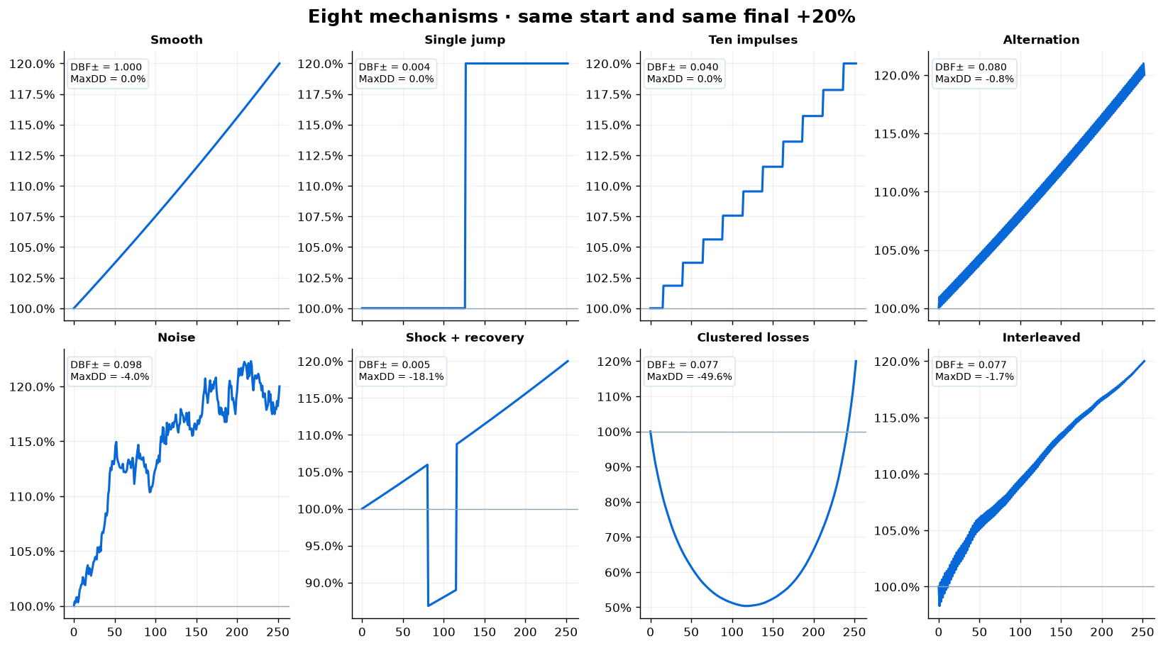
Two strategies may both finish at +20% and reach that destination through very different mechanisms. One may accumulate small gains throughout most of the year; another may earn everything in a single session; a third may alternate large gains and losses before ending at the same point.
Sharpe asks about mean return relative to dispersion; Calmar relates growth to maximum drawdown; the Ulcer Index summarizes drawdown depth and persistence. DBF asks a different question:
Is the net direction supported by many contributions of comparable magnitude, or does it depend on a few observations?
The word breadth is retained deliberately because it does not simply mean “regularity”. It describes the effective fraction of participating magnitudes, not the visual smoothness of the equity curve. The corresponding effective number is N·J=N₂.
2Compact formulation
Let rₜ be the log return in period t, and let N be the total number of observations in the window. The unit may be a day, week, month, or trade, but it must be declared before calculating the metric.
The expression reduces to one fraction:
For an all-zero series we adopt D±=J=DBF±=0. There is no directional information or activity to distribute. This is an explicit computational convention, not an economic claim.
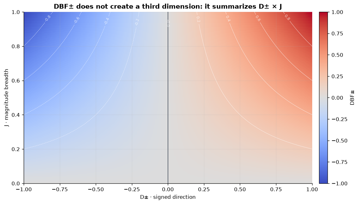
D±=1: every nonzero movement is positive.D±=−1: every nonzero movement is negative.D±=0: positive and negative movement cancel exactly.J=1: every magnitude is equal and no period is zero.J=1/N: one observation concentrates the full magnitude.
3Mathematical anatomy and relationship with Sharpe
DBF does not start from components without precedent. D± is the signed Kaufman Efficiency Ratio applied to the same increments. J is Jain's index applied to |rₜ|; moreover, N·J equals the effective number of order 2 —inverse Herfindahl or Hill N₂— for the weights wₜ=|rₜ|/Σ|rₜ|.
With the periodic Sharpe ratio, zero risk-free rate, and population standard deviation,
the following exact identity holds:
Zero-variance boundary. Sharpe is undefined when variance is exactly zero; the smooth deterministic curve is therefore displayed as ∞, not as a finite ratio. The identity extends to this boundary by continuity as variance tends to zero.
This forces a restrained interpretation: holding J fixed, DBF is a bounded monotonic transformation of Sharpe. Compressing Sharpe creates no new information. Any potential incremental content resides in J, and its economic usefulness still requires out-of-sample validation.
The unsigned version previously published as the Coherence Factor satisfies CF=|DBF±|. DBF preserves sign inside direction itself, without adding a penalty branch or a hyperparameter η.
| D± | J | DBF± | Periodic Sharpe | Identity | Error | |
|---|---|---|---|---|---|---|
| Mechanism | ||||||
| Smooth | 1.0000 | 1.0000 | 1.0000 | ∞ | 1.0000 | 0.0e+00 |
| Single jump | 1.0000 | 0.0040 | 0.0040 | 0.0631 | 0.0040 | 8.7e-19 |
| Ten impulses | 1.0000 | 0.0397 | 0.0397 | 0.2033 | 0.0397 | 0.0e+00 |
| Alternation | 0.0804 | 0.9936 | 0.0799 | 0.0804 | 0.0799 | 2.8e-17 |
| Noise | 0.1549 | 0.6349 | 0.0983 | 0.1243 | 0.0983 | 1.4e-17 |
| Shock + recovery | 0.3139 | 0.0167 | 0.0052 | 0.0406 | 0.0052 | 0.0e+00 |
| Clustered losses | 0.1173 | 0.6524 | 0.0765 | 0.0952 | 0.0765 | 0.0e+00 |
| Interleaved | 0.1173 | 0.6524 | 0.0765 | 0.0952 | 0.0765 | 1.4e-17 |
4Controlled laboratory: same destination, different mechanism
Every curve below finishes at exactly +20%. The number of contributions, cancellation, and order vary. These are not backtests or market samples: they are economic unit tests designed to isolate behavior.
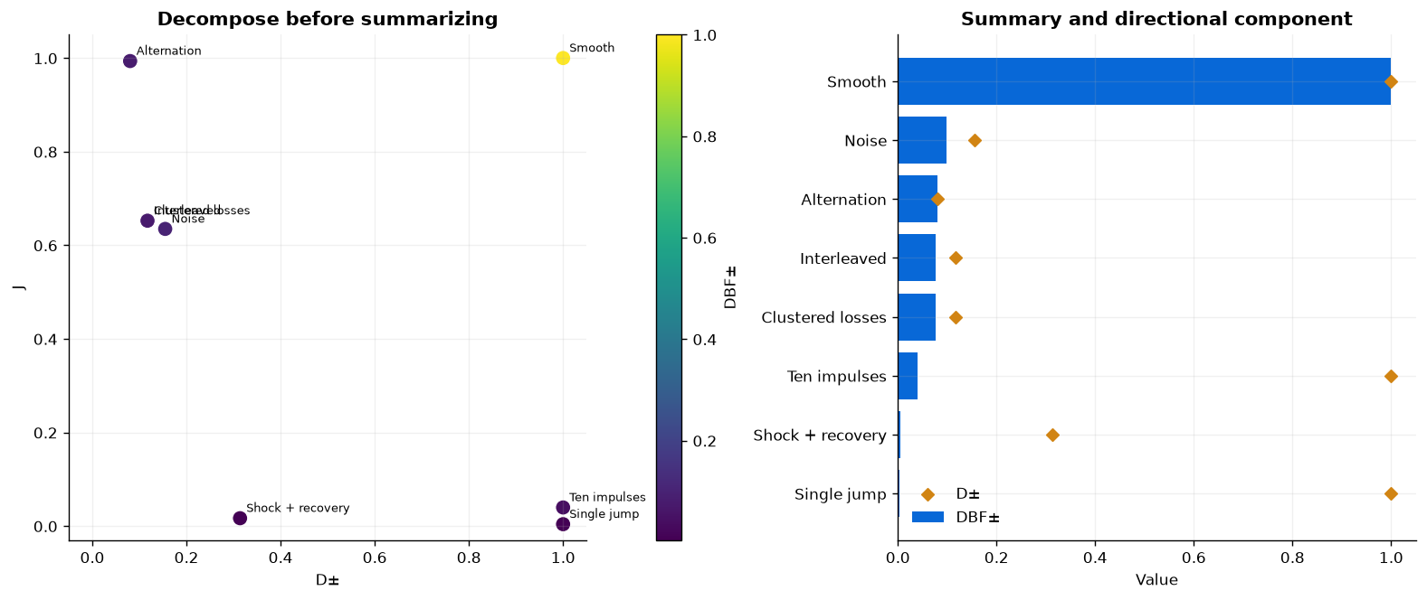
The component view is most informative. A strategy may have high D± and low J —a concentrated directional gain— or high J and low D± —widely distributed activity that cancels. A low DBF does not identify which mechanism dominates on its own.
| CAGR | Sharpe p.a. | Calmar | MaxDD | Ulcer Index | D± | J | DBF± | |
|---|---|---|---|---|---|---|---|---|
| Smooth | 20.00% | ∞ | — | 0.00% | 0.00% | 1.000 | 1.000 | 1.000 |
| Noise | 20.00% | 1.97 | 5.01 | -3.99% | 1.63% | 0.155 | 0.635 | 0.098 |
| Alternation | 20.00% | 1.28 | 24.26 | -0.82% | 0.58% | 0.080 | 0.994 | 0.080 |
| Clustered losses | 20.00% | 1.51 | 0.40 | -49.64% | 38.05% | 0.117 | 0.652 | 0.077 |
| Interleaved | 20.00% | 1.51 | 11.66 | -1.72% | 0.48% | 0.117 | 0.652 | 0.077 |
| Ten impulses | 20.00% | 3.23 | — | 0.00% | 0.00% | 1.000 | 0.040 | 0.040 |
| Shock + recovery | 20.00% | 0.64 | 1.11 | -18.07% | 6.35% | 0.314 | 0.017 | 0.005 |
| Single jump | 20.00% | 1.00 | — | 0.00% | 0.00% | 1.000 | 0.004 | 0.004 |
5What DBF does not observe: temporal order
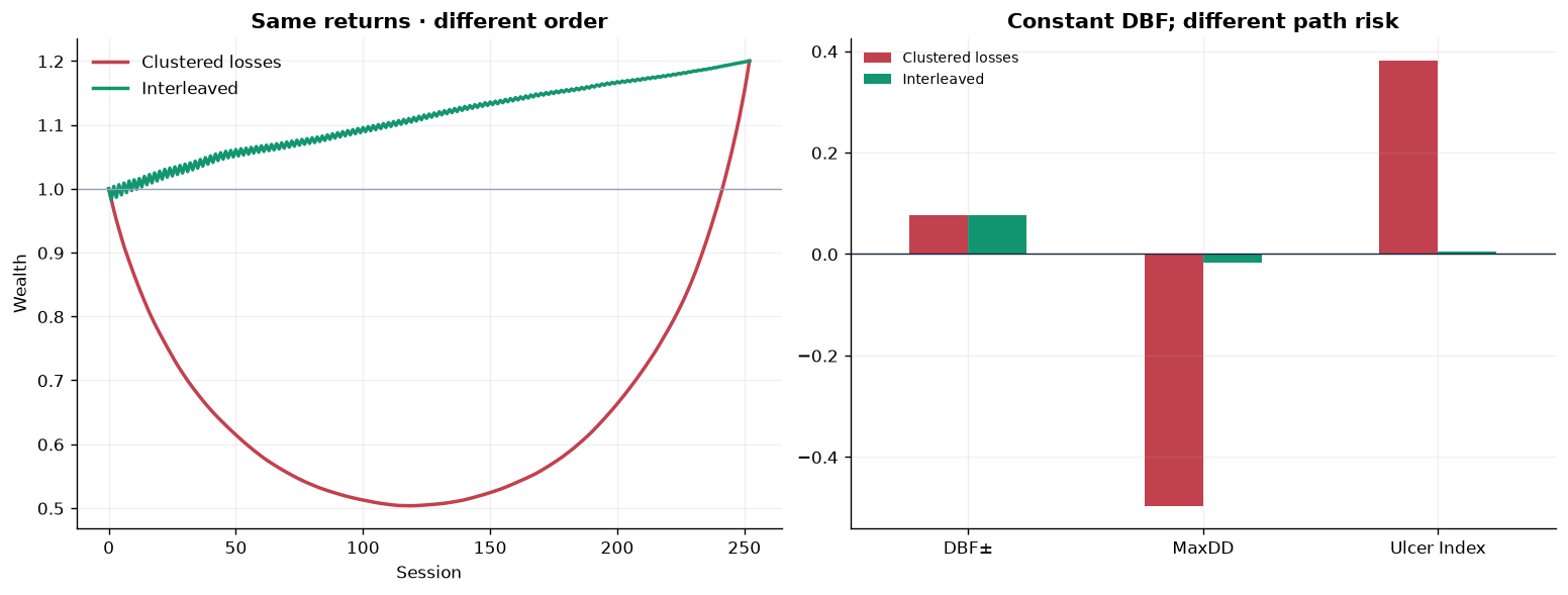
D±, J, Sharpe, and DBF depend on the multiset of returns, not their order. “Clustered losses” and “interleaved” contain exactly the same values and therefore obtain the same DBF by construction. Their drawdowns and economic experiences nevertheless differ.
This is not an implementation bug; it is a boundary of the estimand. Path analysis requires path-aware measures such as maximum drawdown, the Ulcer Index, Martin, or direct inspection of the equity curve.
| CAGR | Sharpe p.a. | D± | J | DBF± | MaxDD | Ulcer Index | |
|---|---|---|---|---|---|---|---|
| Clustered losses | 20.00% | 1.511 | 0.117 | 0.652 | 0.077 | -49.64% | 38.05% |
| Interleaved | 20.00% | 1.511 | 0.117 | 0.652 | 0.077 | -1.72% | 0.48% |
6What DBF also does not observe: economic severity
Preserving sign solves an important presentation problem: a sustained loss no longer appears as “positive coherence”. DBF nevertheless remains scale-invariant. A smooth −0.05% loss and a smooth −90% loss have the same relative pattern and may both produce DBF±=−1.
It means that, for the selected window and frequency, contributions were negative, equal in magnitude, and distributed across every observation. Loss magnitude lives in CAGR or total return.
With losses, two states with the same CAGR may motivate different investigations: a gradual loss with high breadth shows a loss distributed within the window; a single crash with low breadth concentrates the adverse outcome in one event and may justify reviewing tail exposure. DBF describes that historical difference, but it does not identify the edge, measure tail risk on its own, or automatically decide which strategy should be closed or rescued.
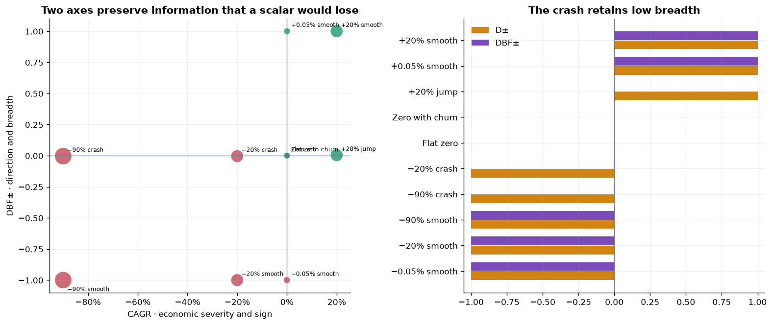
| CAGR | MaxDD | Ulcer Index | D± | J | DBF± | |
|---|---|---|---|---|---|---|
| +0.05% smooth | 0.05% | 0.00% | 0.00% | 1.000 | 1.000 | 1.000 |
| +20% smooth | 20.00% | 0.00% | 0.00% | 1.000 | 1.000 | 1.000 |
| +20% jump | 20.00% | 0.00% | 0.00% | 1.000 | 0.004 | 0.004 |
| Flat zero | 0.00% | 0.00% | 0.00% | 0.000 | 0.000 | 0.000 |
| Zero with churn | 0.00% | -1.00% | 0.70% | 0.000 | 1.000 | 0.000 |
| −0.05% smooth | -0.05% | -0.05% | 0.03% | -1.000 | 1.000 | -1.000 |
| −20% smooth | -20.00% | -20.00% | 11.88% | -1.000 | 1.000 | -1.000 |
| −20% crash | -20.00% | -20.00% | 19.96% | -1.000 | 0.004 | -0.004 |
| −90% smooth | -90.00% | -90.00% | 65.81% | -1.000 | 1.000 | -1.000 |
| −90% crash | -90.00% | -90.00% | 89.82% | -1.000 | 0.004 | -0.004 |
7Frequency is part of the metric
DBF does not exist independently of an observational unit. Twelve positive PnLs spread across twelve trades produce J=1; the same twelve PnLs placed within 252 sessions —with 240 inactive days— produce J=12/252. Neither answer is “the true one” without first defining the question.
Temporal aggregation also changes contributions: daily movements that cancel within a week disappear when weekly PnL is calculated. A daily DBF and a trade-level DBF therefore must not be compared as if they measured exactly the same object.
Frequency sensitivity may reveal useful information about the mechanism, or become a source of arbitrariness if selected after observing the ranking.
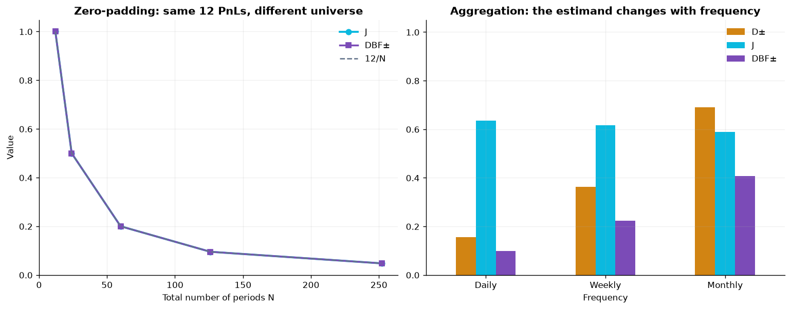
| Active | D± | J | DBF± | |
|---|---|---|---|---|
| N | ||||
| 12 | 12 | 1.000 | 1.000 | 1.000 |
| 24 | 12 | 1.000 | 0.500 | 0.500 |
| 60 | 12 | 1.000 | 0.200 | 0.200 |
| 126 | 12 | 1.000 | 0.095 | 0.095 |
| 252 | 12 | 1.000 | 0.048 | 0.048 |
| Observations | Discarded | D± | J | DBF± | |
|---|---|---|---|---|---|
| Frequency | |||||
| Daily | 252 | 0 | 0.155 | 0.635 | 0.098 |
| Weekly | 50 | 2 | 0.362 | 0.616 | 0.223 |
| Monthly | 12 | 0 | 0.691 | 0.590 | 0.408 |
8Comparison with established industry references
There is no winning metric because each one answers a different question. DBF belongs in a strategy factsheet as a complementary descriptor, not as a replacement for the performance-and-risk core.
| Metric | Primary question | Observes order | Observes absolute severity | Strength | Relevant limitation |
|---|---|---|---|---|---|
| CAGR | How much did capital grow or decline on an annualized basis? | No | Yes | Clear economic magnitude | Does not describe the path |
| Sharpe | What mean return was obtained per unit of dispersion? | No | No; scale-invariant | Familiar and widely comparable standard | Sensitive to assumptions, frequency, and non-Gaussian distributions |
| Sortino | What mean return was obtained per unit of downside deviation? | No | No; scale-invariant | Separates adverse volatility | Depends on the target and ignores sequence |
| Calmar | How much growth was obtained relative to maximum drawdown? | Yes | Yes | Intuitive economic reading | One extreme determines the denominator |
| Ulcer / Martin | How deep and persistent were drawdowns, or how much return compensated for them? | Yes | Yes | Describes the underwater experience | Ulcer is a drawdown level; Martin additionally requires a return convention |
| DBF± | What net direction is supported by breadth? | No | No | Signed, bounded, decomposable, and hyperparameter-free | Requires CAGR, path risk, and a declared frequency |
8.1Reading DBF alongside Sharpe
- Sharpe and DBF share information algebraically; they must not be marketed as orthogonal.
- DBF exposes
J, but it has not yet been shown thatJimproves an out-of-sample decision. - Boundedness in
[−1,1]aids communication but compresses extreme differences. - When the decision requires a scalar economic utility, a utility-derived measure such as MPPM is a more appropriate benchmark than an arbitrary penalty.
| Exact inputs | Output | Direct consequence | |
|---|---|---|---|
| Metric | |||
| CAGR | Initial equity, final equity, and elapsed time | Annualized growth between endpoints | Does not use intermediate values |
| Sharpe | Mean and standard deviation of periodic returns | Mean per unit of dispersion | Order-invariant and positive-scale invariant |
| Sortino | Mean, target, and downside deviation | Mean relative to dispersion below the target | Depends on the selected target |
| Calmar | CAGR and maximum path drawdown | Growth relative to the worst drawdown | One extreme determines the denominator |
| Ulcer Index | Full drawdown series | Quadratic depth below previous highs | Does not include return in the numerator |
| Martin | Return or excess return and Ulcer Index | Growth relative to drawdown pain | Depends on both conventions |
| DBF± | Sum, L1, and L2 of log returns; N | Net direction supported by breadth | Order-invariant and positive-scale invariant |
9Potential uses in quantitative finance
DBF may be useful when the question is specified before observing the result and comparisons are made within homogeneous universes: same frequency, horizon, costs, exposure, and PnL convention.
Flag strategies with similar CAGR but very different dependence on a few dates or trades. This is a prompt for investigation, not a rejection rule.
Separate distributed historical directional outcomes, high cancellation, and event-dominated results.
Compare recent `D±` and `J` with their historical distributions to detect changes in mechanism.
Examine whether aggregate PnL depends on a few temporal contributions or a small number of components.
Force an explicit discussion of frequency, zeros, concentration, and event-driven strategies.
Compare DBF with path-aware measures after reordering or bootstrapping returns to isolate the role of order.
9.1Minimum recommended protocol
- Fix the observational unit and window before calculation.
- Always report
(CAGR, D±, J, DBF±)together with drawdown and costs. - Compare only strategies with compatible exposure and frequency.
- Investigate low
D±and lowJseparately: they imply different mechanisms. - Do not optimize DBF as a standalone objective until an out-of-sample validation tied to a concrete decision exists.
10Python formulation from an array of PnLs
The public function is simply named dbf. It accepts periodic PnLs and the initial capital to which they belong. Capital is required to reconstruct a strictly positive equity curve, transform monetary PnL into log returns, and calculate a comparable CAGR.
10.1Minimal example
If the data are already log returns, the three mathematical expressions may be applied directly. With trade-level PnLs, N is the number of trades; with daily PnLs, inactive days must remain as zeros. Those two estimands are not interchangeable.
The complete reference implementation, tests and executable notebook are maintained in the public GitHub repository linked at the end of this study. This web edition includes only the minimal usage example needed to make the Python contract immediately testable.
from qinvia_direction_breadth_factor import dbf
import numpy as np

pnls = np.array([120.0, -40.0, 90.0, 35.0])
result = dbf(pnls, initial_capital=100_000.0)

print(result["cagr"])
print(result["direction"], result["breadth"])
print(result["dbf_signed"])| cagr | direction | breadth | dbf_signed | dbf | |
|---|---|---|---|---|---|
| 0 | 13.771% | 0.7193 | 0.8016 | 0.5766 | 0.5766 |
11Strengths, limitations, and validation agenda
| Aspect | Candid reading |
|---|---|
| Formulation | Closed-form, bounded, signed, decomposable, and hyperparameter-free |
| Interpretation | Net direction supported by magnitude breadth |
| Order | Permutation-invariant; does not measure path or sequential risk |
| Severity | Scale-invariant; must be paired with CAGR or total return |
| Frequency | Changes under temporal aggregation and zero-padding; the observational unit is part of the definition |
| Sporadic strategies | Low J may indicate fragility or be a legitimate feature of an event-driven style |
| Sharpe | Exact algebraic relationship; potential incremental content lies in J, not in compressing Sharpe |
| Empirical status | Experimental descriptor; no out-of-sample predictive validation yet |
11.1What remains for the paper
This note establishes the formulation, terminology, and a reproducible implementation. Future academic work must study estimator theory, behavior under dependence and heavy tails, statistical power, frequency robustness, and above all whether J adds incremental value to a real out-of-sample decision.
We do not claim that DBF is superior to Sharpe, predicts returns, measures tail risk, is manipulation-proof, or decides on its own which strategy should be retained. Nor do we claim priority over Kaufman, Jain, Hill, effective numbers, Mallart–Fink, or the algebraic identities derived from those components. QINVIA's contribution is this signed synthesis, its terminology, implementation, and joint interpretation.
12References
- Barredo Lago, C. (2026), Beyond Sharpe: TRACE, TRACE Lite and the Coherence Ratio, QINVIA Research.
- Sharpe, W. F. (1994), The Sharpe Ratio, Journal of Portfolio Management.
- Kaufman, P. J. (1995), Smarter Trading, McGraw-Hill.
- Jain, R., Chiu, D. & Hawe, W. (1984), A Quantitative Measure of Fairness and Discrimination for Resource Allocation, DEC TR-301.
- Hill, M. O. (1973), Diversity and Evenness: A Unifying Notation and Its Consequences, Ecology, 54(2), 427–432.
- Mallart, R. & Fink, M. (1994), Adaptive focusing in scattering media through sound-speed inhomogeneities, Journal of the Acoustical Society of America, 96(6), 3721–3732.
- Young, T. W. (1991), “Calmar Ratio: A Smoother Tool”, Futures.
- Martin, P., Ulcer Index and Ulcer Performance Index.
- Goetzmann, W., Ingersoll, J., Spiegel, M. & Welch, I. (2007), Portfolio Performance Manipulation and Manipulation-proof Performance Measures, Review of Financial Studies, 20(5), 1503–1546.
Suggested citation: Barredo Lago, Carlos (2026). “DBF: direction and breadth of the outcome”. QINVIA Technical/Discovery Note 0.1. Not peer reviewed.
GitHub
Code, notebook and reproducible materials.
The public repository preserves the signed DBF implementation, its tests and the executable notebooks. This web publication retains the complete formulation, figures, tables, results, limitations and conclusion.
GitHub Code and reproduction