
Research notebook · Performance measurement
Beyond Sharpe
TRACE, TRACE Lite and the Coherence Ratio: three experimental lenses for describing path, drawdown and concentration beyond traditional ratios.
Executive summary
This study does not attempt to crown a universal ratio. It presents three experimental, descriptive lenses for a concrete question: how can we distinguish two strategies with similar returns but radically different economic experiences? The formulas are published with their strengths, edge cases and code; they are not presented as validated estimators of future returns.
Three experimental lenses
Complementary readings—not a universal ranking—of the same PnL series.
Combines regularity, drawdown and directional concentration; it requires sensitivity analysis and component-level reading.
Summarizes mean distance from a line; it does not replace a risk measure.
Measures direction and magnitude breadth; it ignores order.
1Return, risk and path quality
A return figure tells us how much was gained or lost. It does not tell us whether the result was stable, depended on a single session, required enduring a prolonged drawdown, or whether an apparently clean path concealed continuous cancellation between gains and losses.
The following metrics describe a historical sample. Strategy selection must also consider costs, capacity, tails, dependence, statistical uncertainty and out-of-sample validation.
2What established measures contribute
| Measure | Primary question | Strength | Relevant blind spot |
|---|---|---|---|
| Sharpe | How much excess return is obtained per unit of volatility? | Standard, comparable and connected to allocation under mean–variance assumptions | Treats upside and downside variation symmetrically; ignores order and concentration |
| Sortino | How much return is obtained per unit of downside deviation relative to a target? | Focuses risk on adverse outcomes | Depends on the MAR and can be unstable with few negative observations |
| Calmar | How much CAGR is obtained per unit of maximum drawdown? | Highly intuitive for capital-loss strategies | A single extreme observation dominates; ignores duration and the rest of the path |
| Martin | How much CAGR is obtained per unit of Ulcer Index? | Incorporates the depth and duration of all drawdowns | Can diverge as UI approaches zero; does not measure profit concentration |
| Omega | What is the mass of gains relative to losses around a threshold? | Incorporates the full distribution relative to the threshold | Depends on the threshold and ignores temporal order |
| K-ratio | How significant is the slope of cumulative returns? | A direct precedent for assessing equity-curve regularity | Depends on trend specification, frequency and sample length |
None of these limitations invalidates the measure. Each ratio compresses a different question. The error begins when a partial answer is treated as a universal definition of “quality”.
3From CWR to a multidimensional reading of the path
CWR —Consistency-Weighted Return— was an initial attempt to answer a question that distribution-based ratios do not solve on their own: if two strategies earn the same return, how should we reward the one that gets there more consistently? Its intuition is to multiply return by the fit of the cumulative path to a linear trend.
3.1Intuition and construction
R²₀ is obtained by fitting cumulative arithmetic PnL against time with a line forced through the origin. A path close to that line retains more of its return; an irregular path is discounted. The proposal has two important virtues: it is easy to communicate and places the shape of the equity curve at the center of the analysis.
3.2Why it is not sufficient as a general quality measure
This review does not invalidate the original question. It identifies where one regression compresses economically distinct phenomena:
- Accumulation and apparent fit. Cumulative series are persistent by construction; a high R² may reflect integration rather than a stable source of alpha.
- A line forced through the origin. The result depends on the initial level, horizon and timing of the profit. Earning early and earning late can receive very different readings without changing total PnL.
- Unidentified risks. Maximum drawdown, time under water and concentration in a few sessions are not observable components; if they appear at all, they are mixed into the linear fit.
- Negative domain. Multiplying a loss by a factor between zero and one moves it toward zero. A strategy that loses heavily can therefore appear less bad precisely when its path is worse.
- Frequency and sample length. Moving from daily to monthly data changes the geometry of the regression and therefore its reading of consistency.
3.3The role of CWR in this study
CWR remains a historical reference and conceptual starting point, not an opponent to defeat. TRACE retains the multidimensional ambition, TRACE Lite reformulates regularity through geometric distance, and the Coherence Ratio separates direction and concentration in closed form. The main evolution is to expose the components and define consistently what happens when the outcome is negative.
4Three experimental lenses
4.1TRACE
TRACE stands for Trajectory, Risk, Alignment and Concentration Efficiency. The name reflects its three blocks: path regularity, drawdown risk and the alignment/concentration of contributions. Let R = CAGR:
P_R: proximity to the log-linear path, regularized by variability.U = 1/(1+UI/u₀): a drawdown factor based on the Ulcer Index.Cdir: distribution of contributions aligned with the sign of the outcome.
The negative branch differs because multiplying a loss by a factor below one would move it toward zero and reward a worse path. This study uses γ=δ=λ=η=1 and u₀=10% by default; these values must be disclosed and sensitivity-tested.
Status and limitation. TRACE is a heuristic composite, not a ratio derived from a statistical theory. P_R, U and Cdir may overlap; P_R uses a normalization in which greater variability also enlarges the denominator, while Cdir evaluates only aligned contributions rather than the full set of available periods. The score should therefore always be reported with its components and used as a secondary diagnostic, not as a single optimization objective.
4.2TRACE Lite
If xₜ = log(Eₜ) and aₜ is the line joining the initial and terminal values:
It is easy to communicate and requires no calibration, although a visually straight cumulative curve may conceal returns that continuously cancel one another. Moreover, because the distance is averaged across the full sample, a very brief crash can be diluted and coexist with a high LQ. TRACE Lite is a geometric baseline, not a sufficient measure of drawdown, concentration or tail risk.
4.3Coherence Factor and Coherence Ratio
For log returns ℓₜ:
This expression equals D × J: directional efficiency D=|Σℓₜ|/Σ|ℓₜ| times Jain applied to magnitudes J=(Σ|ℓₜ|)²/(NΣℓₜ²). CF=1 requires equal movements in one direction; a single impulse produces CF=1/N; cancellation pushes CF toward zero. N·J=1/Σwₜ², where wₜ=|ℓₜ|/Σ|ℓₜ|, is algebraically an effective number or inverse Herfindahl. In the academic line we use the more precise name Direction–Breadth Factor (DBF); this article retains Coherence Factor for editorial continuity.
CF is dimensionless; the Coherence Ratio retains return units. Despite its public name, Coherence Ratio is mathematically a signed score, not a statistical ratio or a realizable return. Its negative branch uses the normative choice η=1 and may produce values below −100%. The more transparent primary reading is the pair (CAGR, CF); the score is a secondary summary.
CF is order-invariant: it does not distinguish when returns occurred. J combines inactive periods and unequal magnitudes, so it does not by itself separate sparsity, tails and concentration. It also changes with zero-padding and frequency, and may penalize legitimately sporadic alpha.
5Experimental design
The study uses two synthetic laboratories:
- Same outcome: 16 curves finish at 1.25 after 504 sessions. CAGR is identical; only geometry, volatility, concentration, autocorrelation and order change.
- Signed domain: 11 one-year curves span +25%, zero and losses down to −90%, including smooth, volatile and single-jump or single-crash paths.
The curves are not intended to imitate a specific strategy. They are economic unit tests that make one dominant property visible, but they are not a factorial design, a causal estimate or empirical validation. Matching the terminal value modifies each series' drift; the results should be read as a controlled diagnostic gallery.
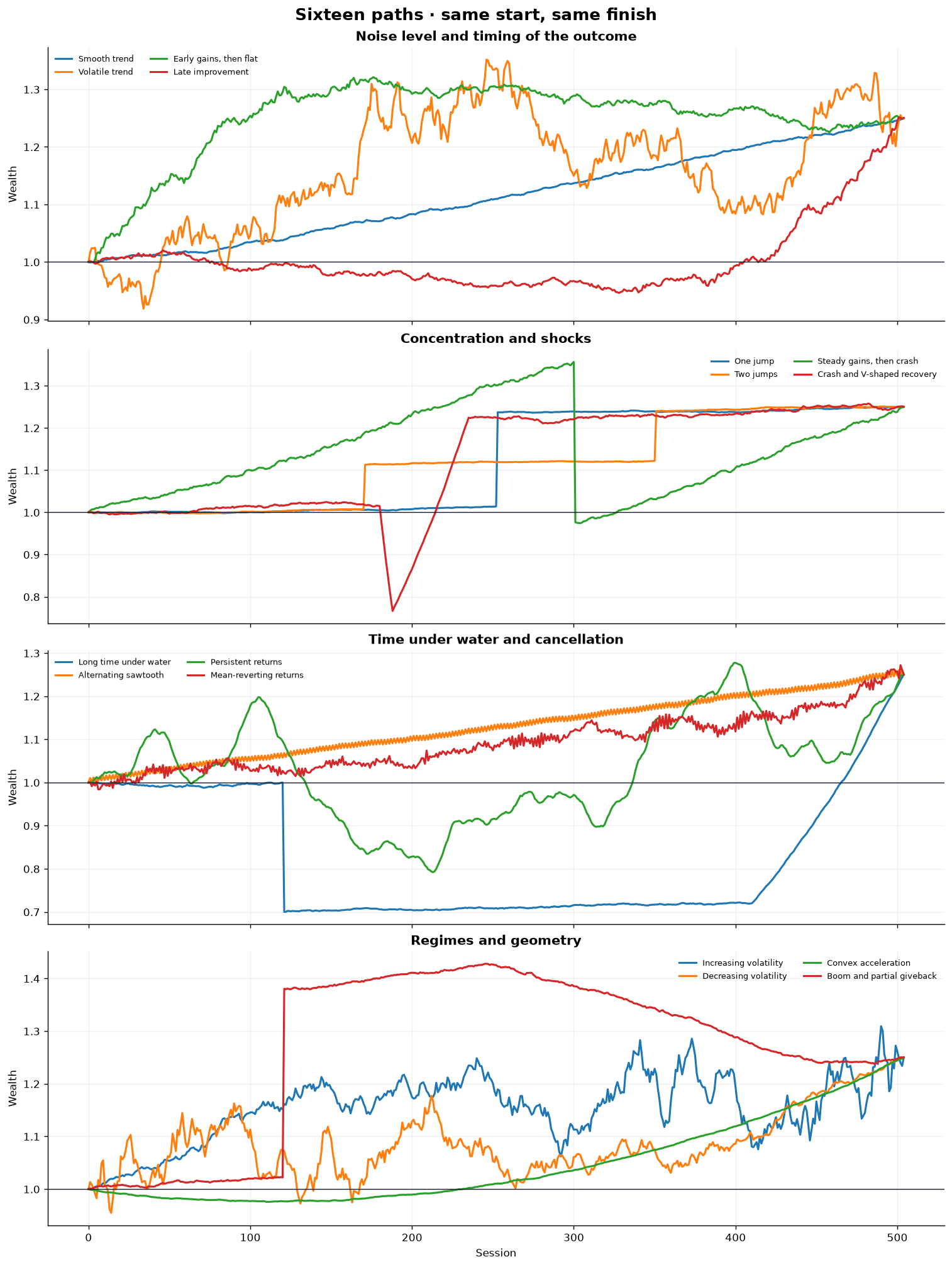
| CAGR | Max drawdown | Ulcer Index | R2 origin | P_R | U | Cdir | Q_TRACE | LQ | CF | |
|---|---|---|---|---|---|---|---|---|---|---|
| Smooth trend | 11.80% | 0.28% | 0.06% | 0.997 | 0.968 | 0.994 | 0.994 | 0.957 | 0.974 | 0.435 |
| Volatile trend | 11.80% | 19.90% | 9.12% | 0.837 | 0.811 | 0.523 | 0.989 | 0.419 | 0.837 | 0.030 |
| Early gains, then flat | 11.80% | 7.27% | 3.31% | 0.797 | 0.646 | 0.751 | 0.985 | 0.478 | 0.610 | 0.110 |
| Late improvement | 11.80% | 7.27% | 3.93% | 0.071 | 0.646 | 0.718 | 0.985 | 0.457 | 0.610 | 0.110 |
| One jump | 11.80% | 0.45% | 0.14% | 0.862 | 0.838 | 0.986 | 0.292 | 0.242 | 0.778 | 0.004 |
| Two jumps | 11.80% | 0.33% | 0.10% | 0.944 | 0.888 | 0.990 | 0.646 | 0.568 | 0.875 | 0.007 |
| Steady gains, then crash | 11.80% | 28.17% | 12.25% | 0.775 | 0.805 | 0.449 | 0.994 | 0.360 | 0.753 | 0.004 |
| Crash and V-shaped recovery | 11.80% | 25.20% | 4.08% | 0.798 | 0.772 | 0.710 | 0.986 | 0.541 | 0.895 | 0.034 |
| Long time under water | 11.80% | 30.07% | 22.64% | 0.392 | 0.534 | 0.306 | 0.992 | 0.162 | 0.452 | 0.004 |
| Alternating sawtooth | 11.80% | 1.02% | 0.65% | 0.997 | 0.972 | 0.939 | 1.000 | 0.912 | 0.968 | 0.045 |
| Persistent returns | 11.80% | 33.89% | 17.04% | 0.129 | 0.640 | 0.370 | 0.991 | 0.235 | 0.759 | 0.063 |
| Mean-reverting returns | 11.80% | 4.49% | 1.69% | 0.977 | 0.914 | 0.856 | 0.990 | 0.774 | 0.894 | 0.032 |
| Increasing volatility | 11.80% | 16.36% | 6.33% | 0.857 | 0.836 | 0.612 | 0.982 | 0.503 | 0.798 | 0.030 |
| Decreasing volatility | 11.80% | 16.36% | 8.06% | 0.835 | 0.836 | 0.554 | 0.982 | 0.455 | 0.798 | 0.030 |
| Convex acceleration | 11.80% | 2.45% | 1.17% | 0.697 | 0.750 | 0.895 | 0.995 | 0.668 | 0.725 | 0.500 |
| Boom and partial giveback | 11.80% | 13.33% | 6.32% | 0.787 | 0.700 | 0.613 | 0.332 | 0.142 | 0.654 | 0.003 |
6Comparative results
Absolute values from different ratios are not directly comparable. The heatmap uses within-column percentiles: it shows which paths each definition favors; it does not imply that 0.8 in one metric equals 0.8 in another.
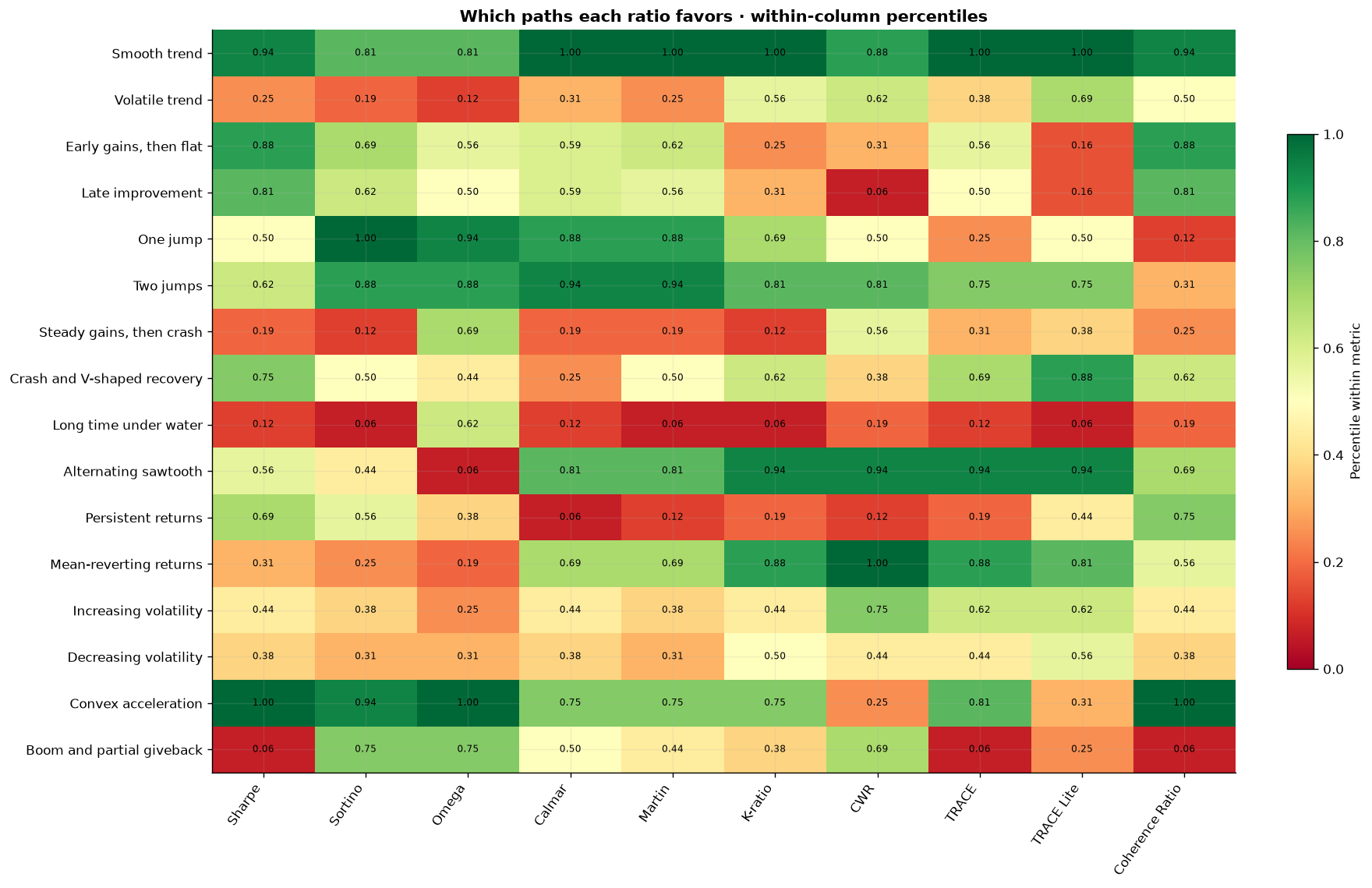
| CAGR | TRACE | TRACE Lite | CF | Coherence Ratio | CWR | Sharpe | Calmar | Martin | K-ratio | |
|---|---|---|---|---|---|---|---|---|---|---|
| Smooth trend | 0.118 | 0.113 | 0.115 | 0.435 | 0.051 | 0.111 | 10.096 | 42.443 | 195.943 | 13.082 |
| Alternating sawtooth | 0.118 | 0.108 | 0.114 | 0.045 | 0.005 | 0.123 | 0.800 | 11.570 | 18.084 | 8.315 |
| Mean-reverting returns | 0.118 | 0.091 | 0.106 | 0.032 | 0.004 | 0.124 | 0.727 | 2.627 | 6.998 | 2.342 |
| Convex acceleration | 0.118 | 0.079 | 0.086 | 0.500 | 0.059 | 0.078 | 12.113 | 4.817 | 10.076 | 1.560 |
| Two jumps | 0.118 | 0.067 | 0.103 | 0.007 | 0.001 | 0.110 | 1.112 | 36.058 | 119.862 | 2.160 |
| Crash and V-shaped recovery | 0.118 | 0.064 | 0.106 | 0.034 | 0.004 | 0.092 | 1.340 | 0.468 | 2.895 | 0.941 |
| Increasing volatility | 0.118 | 0.059 | 0.094 | 0.030 | 0.004 | 0.108 | 0.739 | 0.721 | 1.864 | 0.484 |
| Early gains, then flat | 0.118 | 0.056 | 0.072 | 0.110 | 0.013 | 0.090 | 2.408 | 1.623 | 3.563 | 0.332 |
| Late improvement | 0.118 | 0.054 | 0.072 | 0.110 | 0.013 | 0.008 | 2.408 | 1.623 | 3.002 | 0.338 |
| Decreasing volatility | 0.118 | 0.054 | 0.094 | 0.030 | 0.004 | 0.105 | 0.739 | 0.721 | 1.465 | 0.486 |
| Volatile trend | 0.118 | 0.049 | 0.099 | 0.030 | 0.004 | 0.108 | 0.700 | 0.593 | 1.294 | 0.544 |
| Steady gains, then crash | 0.118 | 0.042 | 0.089 | 0.004 | 0.001 | 0.106 | 0.680 | 0.419 | 0.963 | 0.192 |
| One jump | 0.118 | 0.029 | 0.092 | 0.004 | 0.000 | 0.105 | 0.784 | 26.485 | 85.699 | 1.318 |
| Persistent returns | 0.118 | 0.028 | 0.090 | 0.063 | 0.007 | 0.015 | 1.288 | 0.348 | 0.693 | 0.252 |
| Long time under water | 0.118 | 0.019 | 0.053 | 0.004 | 0.000 | 0.055 | 0.651 | 0.393 | 0.521 | -0.082 |
| Boom and partial giveback | 0.118 | 0.017 | 0.077 | 0.003 | 0.000 | 0.108 | 0.550 | 0.885 | 1.868 | 0.406 |
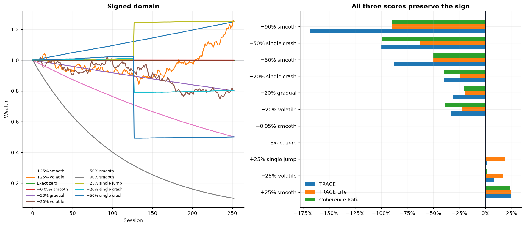
| CAGR | Max drawdown | Ulcer Index | Q_TRACE | LQ | CF | TRACE | TRACE Lite | Coherence Ratio | CWR | |
|---|---|---|---|---|---|---|---|---|---|---|
| +25% smooth | 25.00% | -0.00% | 0.00% | 0.990 | 0.993 | 0.954 | 24.74% | 24.83% | 23.86% | 22.32% |
| +25% volatile | 25.00% | 19.09% | 9.02% | 0.334 | 0.654 | 0.063 | 8.35% | 16.35% | 1.56% | 0.10% |
| Exact zero | 0.00% | -0.00% | 0.00% | 0.000 | 1.000 | 0.000 | 0.00% | 0.00% | 0.00% | — |
| −0.05% smooth | -0.05% | 0.05% | 0.03% | 0.994 | 0.998 | 0.989 | -0.05% | -0.05% | -0.05% | -0.05% |
| −20% gradual | -20.00% | 20.00% | 11.78% | 0.455 | 0.994 | 0.952 | -30.90% | -20.12% | -20.97% | -22.30% |
| −20% volatile | -20.00% | 26.56% | 14.00% | 0.353 | 0.879 | 0.057 | -32.94% | -22.42% | -38.87% | -18.05% |
| −50% smooth | -50.00% | 50.00% | 31.22% | 0.241 | 0.996 | 0.995 | -87.93% | -50.18% | -50.25% | -69.22% |
| −90% smooth | -90.00% | 90.00% | 65.82% | 0.132 | 1.000 | 1.000 | -168.14% | -90.02% | -90.04% | -229.21% |
| +25% single jump | 25.00% | 0.05% | 0.01% | 0.053 | 0.760 | 0.005 | 1.32% | 19.00% | 0.11% | 21.14% |
| −20% single crash | -20.00% | 22.05% | 15.11% | 0.033 | 0.753 | 0.005 | -39.34% | -24.93% | -39.91% | -15.85% |
| −50% single crash | -50.00% | 52.05% | 36.44% | 0.003 | 0.751 | 0.004 | -99.84% | -62.46% | -99.80% | -39.31% |
6.1What disagreements reveal
- One jump: TRACE and the Coherence Ratio penalize it through concentration; TRACE Lite only sees the distance from the equity curve to a line and is less severe.
- Alternating sawtooth: the cumulative curve may look clean —high LQ— while CF falls because returns continuously cancel one another.
- Increasing and decreasing volatility: CF is identical because the multiset of returns is the same; TRACE can distinguish them through the drawdown path.
- Long time under water: Martin and TRACE penalize it naturally; a purely distributional measure does not know the temporal duration of pain.
- Sporadic strategies: CF assigns
1/Nto a single impulse. This is transparent, but it may reject legitimately sparse alpha such as convex or event-driven payoffs.
These differences suggest a better practice than choosing a champion: use TRACE as a composite diagnostic, TRACE Lite as a geometric baseline, and the pair (CAGR, CF) as a description of direction and breadth. The Coherence Ratio may be shown as a secondary signed summary, not as a substitute for its two components.
7Invariances and limits
A publishable metric should state not only what it calculates, but also which transformations leave it unchanged.
| CAGR | Sharpe | Omega | CF | Coherence Ratio | LQ | TRACE | Martin | CWR | |
|---|---|---|---|---|---|---|---|---|---|
| Gains first | 0.118 | 2.408 | 1.509 | 0.110 | 0.013 | 0.610 | 0.056 | 3.563 | 0.090 |
| Gains last | 0.118 | 2.408 | 1.509 | 0.110 | 0.013 | 0.610 | 0.054 | 3.002 | 0.008 |
| Observations | CF | LQ | Ulcer Index | |
|---|---|---|---|---|
| Frequency | ||||
| Daily | 504 | 0.030 | 0.837 | 9.12% |
| Weekly | 100 | 0.061 | 0.820 | 8.65% |
| Monthly | 24 | 0.165 | 0.805 | 8.16% |
| Quarterly | 8 | 0.303 | 0.799 | 8.19% |
| Property | TRACE | TRACE Lite | Coherence Factor / Ratio |
|---|---|---|---|
| Preserves the sign | Yes | Yes | Yes |
| Observes order | Yes | Yes | No |
| Explicitly penalizes drawdown | Yes | Indirectly | No |
| Detects a single jump | Yes | Partly | Yes, extremely |
| Hyperparameters | γ, δ, λ, u₀, η |
None | None |
| Invariant to monetary scale | Yes | Yes | Yes |
| Sensitive to frequency | Yes | Yes | Yes |
| Communication complexity | High | Low | Low |
Common limitation: none of the three formulas estimates uncertainty, corrects for multiple selection or establishes persistence. A high historical score is not a probability of future success.
7.1Known edge cases
| Lens | Case requiring caution | Practical implication |
|---|---|---|
| TRACE | P_R may improve when variability also enlarges its denominator; Cdir conditions on aligned contributions and may not reflect how many periods sustain the outcome |
Read P_R, U and Cdir separately; do not interpret Q_TRACE as a probability or optimize it in isolation |
| TRACE Lite | A one-session flash crash can be diluted in the mean distance and leave LQ high |
Always pair it with maximum drawdown, Ulcer Index and extreme-event diagnostics |
| CF / Coherence Ratio | CF ignores order; J mixes sparsity and unequal magnitudes; the signed transformation with η=1 is normative |
Report (CAGR, CF) first and study frequency, zeros and event-driven styles before using the score |
8Potential uses in quantitative finance
These metrics do not attempt to forecast the next return. Their potential value is to describe, compare and monitor how PnL is generated, which matters when several models display similar aggregate returns.
| Quantitative application | How it would be used | Particularly useful metric | Decision informed |
|---|---|---|---|
| Backtest screening | Compare strategies with similar CAGR and flag paths dependent on one avoided crash or a few sessions for review | TRACE and its components | Which candidates require further validation; not an automatic rejection |
| Model diagnosis | Separate geometric irregularity, drawdown and concentration into auditable components | TRACE and TRACE Lite | Why a strategy receives a low assessment |
| Walk-forward validation | Measure each training and test window, not only the full sample | All three | Whether the descriptor is stable out of sample, not whether it predicts on its own |
| Production monitoring | Calculate rolling windows and compare their distribution with the backtest | TRACE Lite and (CAGR, CF) |
A descriptive alert of possible drift that must then be investigated |
| Ensemble construction | Flag sleeves whose profit depends on very few observations or strong internal cancellation | CF and its components D, J |
Where to study concentration or temporal diversification before imposing limits |
| Meta-model features | Use P_R, U, Cdir, LQ and CF as variables, always without future information |
Components, not only scores | Whether path quality adds incremental signal |
| Path stress testing | Reorder or bootstrap returns while approximately preserving the distribution, then remeasure | TRACE versus CF | How much the diagnosis depends on temporal order |
8.1A reasonable workflow
- Report CAGR, volatility, maximum drawdown, Ulcer Index, Sharpe and Calmar first.
- Add TRACE, TRACE Lite and
(CAGR, CF)as a second experimental diagnostic layer; keep the Coherence Ratio as an optional signed summary. - Compare in-sample, out-of-sample and rolling windows; one figure for the entire history conceals regime changes.
- Repeat the analysis across several frequencies and economically coherent initial-capital assumptions.
- Test whether the metrics improve a real decision —selection, limits or allocation— relative to a baseline model that does not use them.
8.2Uses to avoid
They should not become a single optimization objective, an automatic acceptance/rejection rule or a directly realizable “risk-adjusted return”: doing so would encourage overfitting to the formula itself. Nor do they replace costs, capacity, factor exposure, inter-strategy correlation, tails or statistical uncertainty. A high historical score is a descriptive observation, not a probability of future profitability.
9Practical comparison with reference ratios
Established ratios and the new proposals answer different questions. The useful comparison is not to declare a winner, but to identify which dimension is visible and which remains outside the formula.
| Measure | Core question | Observes order | Explicit drawdown | Explicit concentration | Primary use |
|---|---|---|---|---|---|
| Sharpe | How much excess return is obtained per unit of volatility? | No | No | No | Risk–return comparability and portfolio construction |
| Sortino | How much return is obtained per unit of downside deviation? | No | No | No | Strategies with asymmetric outcomes relative to a target |
| Calmar | How much CAGR compensates for the worst drawdown? | Partly | Maximum | No | Strategies where maximum capital loss matters |
| Martin | How much CAGR compensates for drawdown depth and duration? | Yes | Ulcer Index | No | Penalizing prolonged time under water |
| Omega | What mass of gains exceeds losses relative to a threshold? | No | No | No | Non-Gaussian distributions relative to a MAR |
| K-ratio | How statistically stable is the cumulative slope? | Yes | No | No | Regression-based trend regularity |
| TRACE | What signed score results from combining CAGR with regularity, drawdown and concentration? | Yes | Ulcer Factor | Yes | Composite diagnosis and secondary screening |
| TRACE Lite | How close is log equity to its ideal path between endpoints? | Yes | Indirect | No | Geometric explanation and simple monitoring |
| CF / Coherence Ratio | What direction and magnitude breadth are present, and what signed score results when combined with CAGR? | No | No | Yes | Describing cancellation and dependence on few observations |
9.1Strengths and potential weaknesses of our proposals
| Proposal | Main strength | Potential weakness | Most defensible use |
|---|---|---|---|
| TRACE | Makes three dimensions explicit and treats losses monotonically: a worse loss produces a more negative score | Composite with hyperparameters; P_R, U and Cdir may overlap and have their own edge cases |
Research tool, secondary ranking and component-auditable backtest diagnosis |
| TRACE Lite | Transparent, hyperparameter-free and sensitive to temporal order | Its reference is geometric; it can dilute a flash crash and does not detect concentration on its own | Communication, sanity checks and rolling equity-shape monitoring alongside drawdown metrics |
| CF / Coherence Ratio | Closed form decomposable into direction D and breadth J |
CF ignores order and mixes sparsity with inequality; the signed score is normative and not a realizable return | Concentration/cancellation descriptor, control feature and complement to Sharpe/Calmar |
An operational report can keep CAGR, Sharpe, Calmar and Ulcer Index at its core; add TRACE as a composite diagnostic, TRACE Lite to explain geometry, and the pair (CAGR, CF) to reveal cancellation or concentration. Signed scores remain secondary summaries.
10Reproducible implementation
The three public functions share the same inputs: a np.ndarray of periodic PnLs and their initial capital. Capital converts monetary PnL into comparable equity, CAGR and drawdown.
The complete TRACE, TRACE Lite and Coherence Ratio implementation—including input validation, signed treatment, the minimal example and tests—is maintained in the public GitHub repository linked at the end of this study.
11References
- Barredo Lago, C. (2023), Introducing the Consistency-Weighted Return (CWR).
- Sharpe, W. F. (1994), The Sharpe Ratio, Journal of Portfolio Management.
- Sortino, F. A. & van der Meer, R. (1991), Downside Risk, Journal of Portfolio Management, 17(4), 27–31.
- Keating, C. & Shadwick, W. F. (2002), A Universal Performance Measure.
- Martin, P., Ulcer Index and UPI.
- Young, T. W. (1991), “Calmar Ratio: A Smoother Tool”, Futures. · Calmar ratio context
- Kestner, L. N. (2013), (Re)Introducing the K-Ratio.
- Kaufman, P. J. (1995), Smarter Trading, McGraw-Hill.
- Jain, R., Chiu, D. & Hawe, W. (1984), A Quantitative Measure of Fairness and Discrimination for Resource Allocation, DEC TR-301.
- Hill, M. O. (1973), Diversity and Evenness: A Unifying Notation and Its Consequences, Ecology, 54(2), 427–432.
- Mallart, R. & Fink, M. (1994), Adaptive focusing in scattering media through sound-speed inhomogeneities, Journal of the Acoustical Society of America.
TRACE, TRACE Lite and the signed transformation published as Coherence Ratio are working proposals of this study. The Coherence Factor combines directional efficiency with Jain's index applied to magnitudes; its components and the effective-number interpretation have explicit precedents. The public name is retained for continuity, without claiming academic priority or predictive validation.
Reproducible methodological research. This is not financial advice or evidence of future profitability.
GitHub
Code, notebook and reproducible materials.
The public repository preserves the notebook and reference implementation. This web publication retains the complete methods, formulas, figures, results, limitations and conclusion of the study.
GitHub Code and reproduction