
Research note · Statistical arbitrage
Pairs Trading from Scratch: When TRUMP and MELANIA Argue, the Spread Keeps Score
A visual introduction to linear relationships, residuals, Z-scores, OLS, Kalman filters and cointegration—without needless jargon, using real data and a thematic pair that is hard to beat.
The intuition
1A pairs strategy does not predict the market: it compares two things
A directional strategy asks: “Will TRUMP rise?”. A pairs strategy asks a different question: “Has TRUMP become too expensive relative to MELANIA, given the relationship they had been maintaining?”. It can make money even if both cryptocurrencies fall, provided their relative relationship moves in the expected direction.
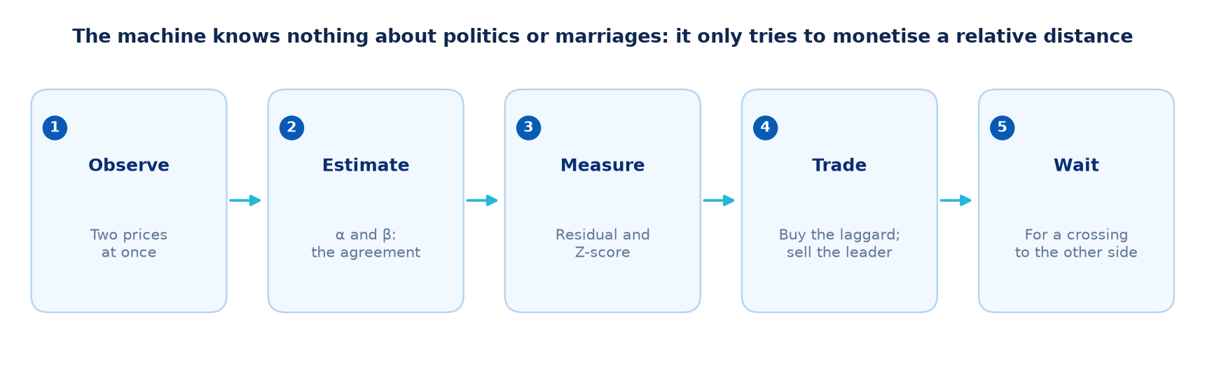
No: the model is not trying to predict who wins an election or who sleeps on the sofa. It only asks whether two prices that usually move together have separated more than usual.
1 · Relationship
We estimate how much TRUMP usually accompanies one unit of MELANIA.
2 · Deviation
We measure how far the observed price moves from the price implied by that relationship.
3 · Convergence
We buy the relatively cheap leg and sell the expensive one, expecting the gap to narrow.
The hypothesis is not “they share a theme, therefore it will work.” The narrative merely proposes a candidate. The data must show a repeatable relationship that remains exploitable after costs.
The real example
2TRUMP and MELANIA: the perfect narrative pair… to put to the test
The example uses the perpetual contracts TRUMPUSDT and MELANIAUSDT on Binance. TRUMP began trading on 18 January 2025; MELANIA on 20 January 2025. The common sample starts when the second contract exists. No earlier history is invented.
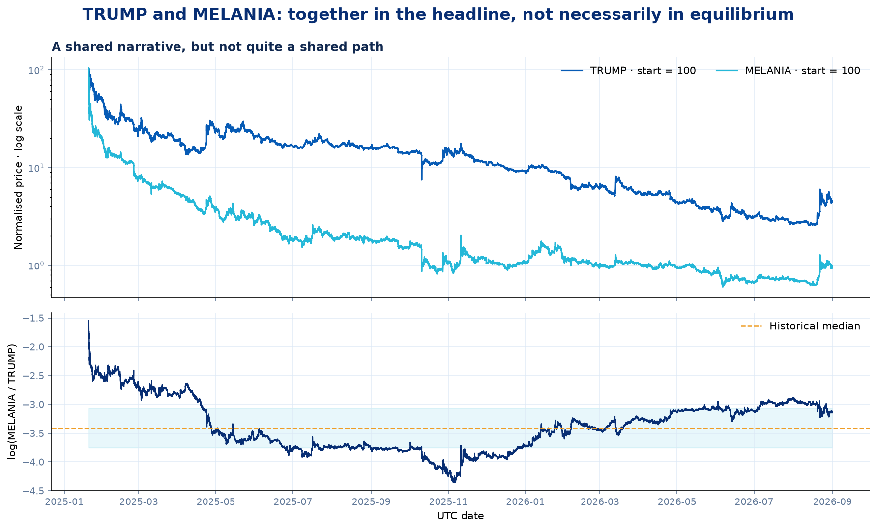
Why Binance when the main research programme uses OKX? Because MELANIA is not currently listed as an active perpetual on OKX, while both contracts are active on Binance. This didactic example remains separate from the main research programme on the OKX universe.
The statistical contract
3The line, the agreement, and the bill for the argument
We call Y the price of MELANIA and X the price of TRUMP. The model attempts to explain Y through X:
β · proportion
If β = 0.03, one unit of MELANIA is hedged with approximately 0.03 units of TRUMP. It is the slope of the relationship.
α · baseline
It allows the line not to pass through the origin. That adds flexibility—and another moving part.
Residual · distance
It is what MELANIA is worth minus what the model says it should be worth. This is the object we expect to revert.
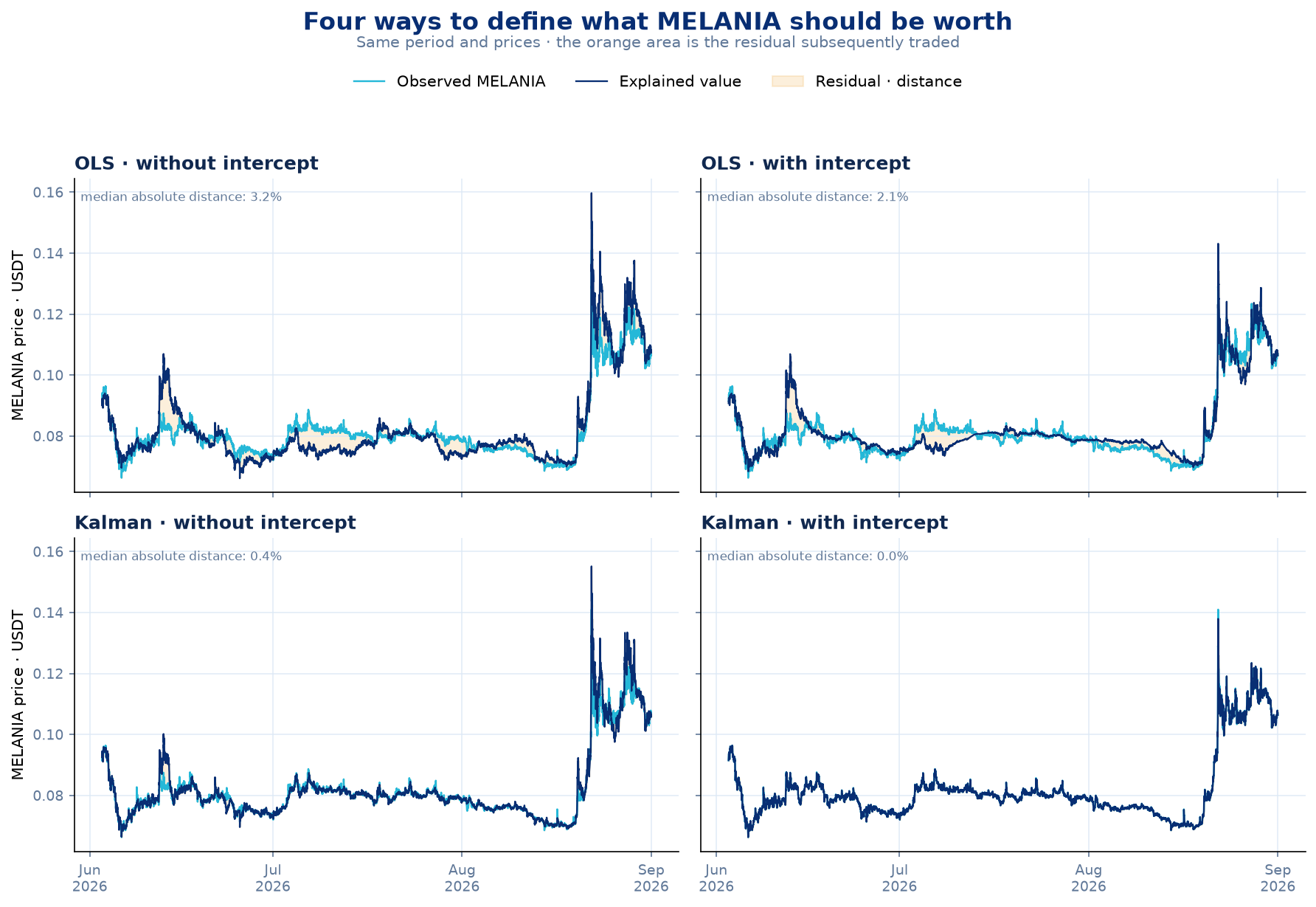
One global line would hide changes in the relationship. We therefore compare, over the same period, how the four models translate TRUMP's price into an explained value for MELANIA. The larger the orange area, the larger the discrepancy the strategy would try to monetise.
The four lines, with the geometry in plain sight
To see the linear relationship literally, we freeze each model's coefficients at the final bar. The points are observations from the last 90 days aggregated to four hours. In OLS and Kalman without an intercept, the line must pass through the origin; with an intercept, α can shift it.
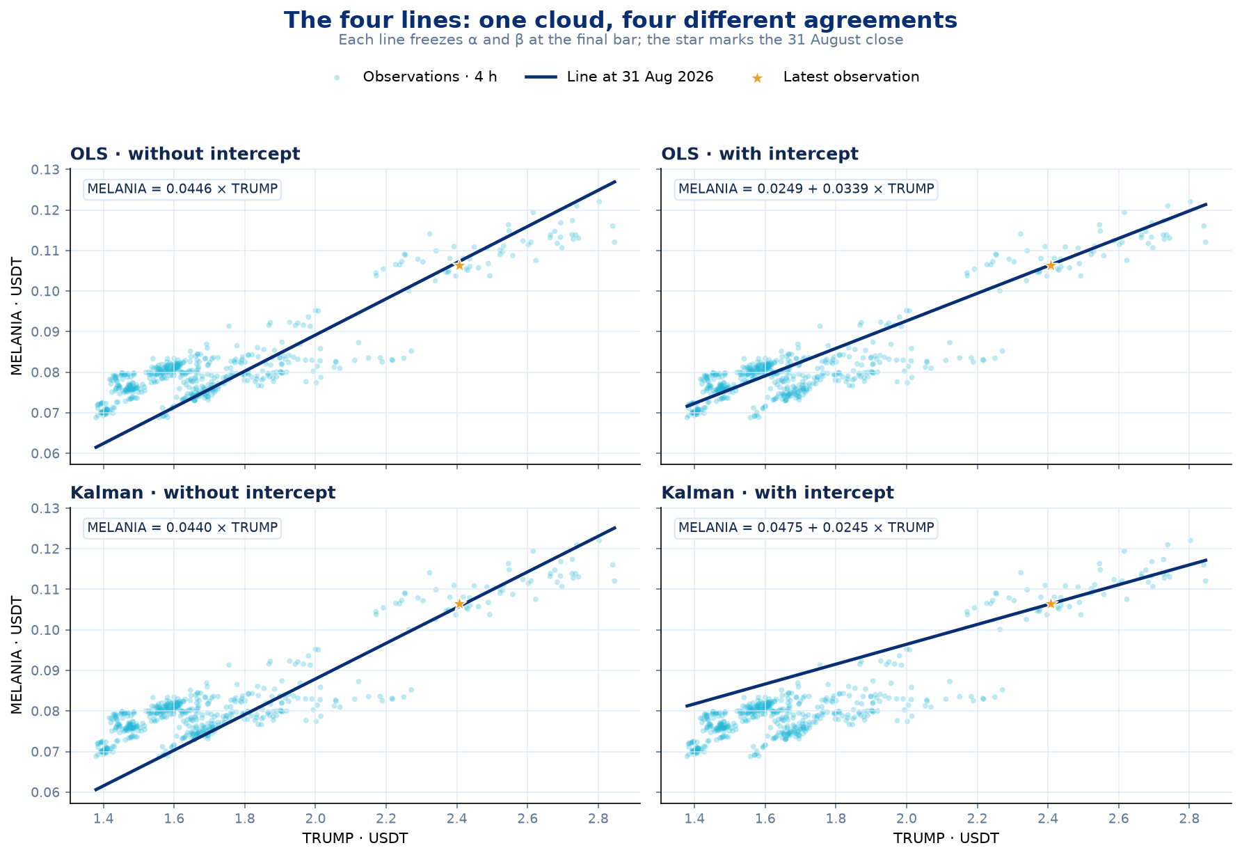
Core idea: β does not try to “predict” the exact price. It builds a relative comparison. The residual is the unsettled bill; the Z-score tells us whether that bill is small or extraordinary relative to its recent history.
Four ways to estimate the relationship
4The same couple, four quantitative therapists
OLS re-estimates a line using a 14-day rolling window. Kalman updates the relationship bar by bar and allows it to change gradually. Without an intercept, qβ = 3·10−8; with an intercept, qβ = 3·10−6 and qα = 3·10−8. In all four cases, the residual is normalised using a 14-day Z-score. These values are illustrative, not optimised.
OLS without intercept
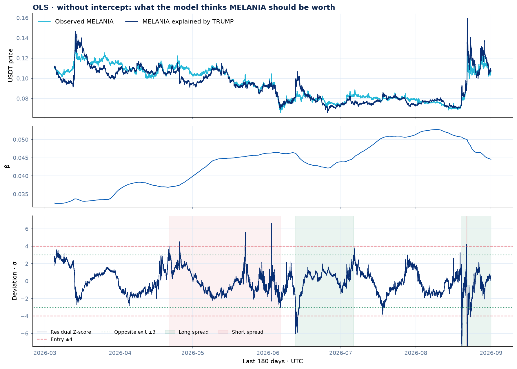
It forces the relationship through the origin: Y = βX. It is simple, stable, and easy to interpret. It may be too rigid when a persistent baseline exists.
OLS with intercept
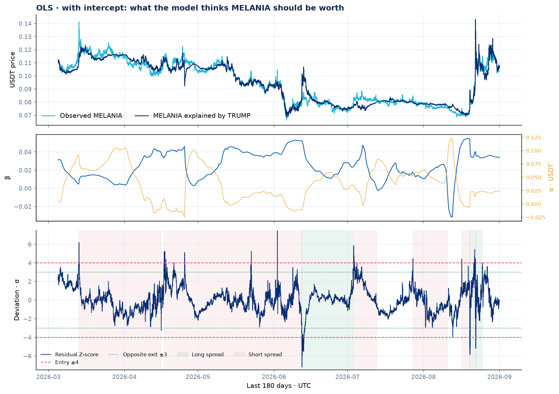
It estimates Y = α + βX. It adapts better to level shifts, but α and β may divide the explanation between them in unstable ways.
Kalman without intercept
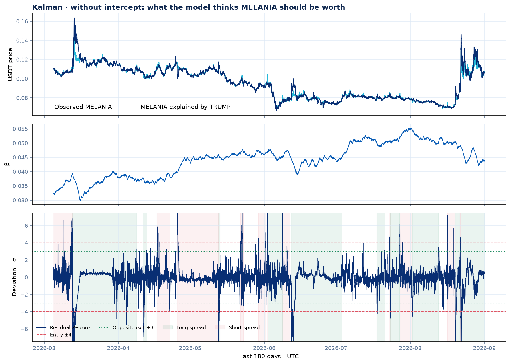
It retains Y = βtX, but allows β to evolve smoothly. It reacts to regime changes; it can also chase noise.
Kalman with intercept
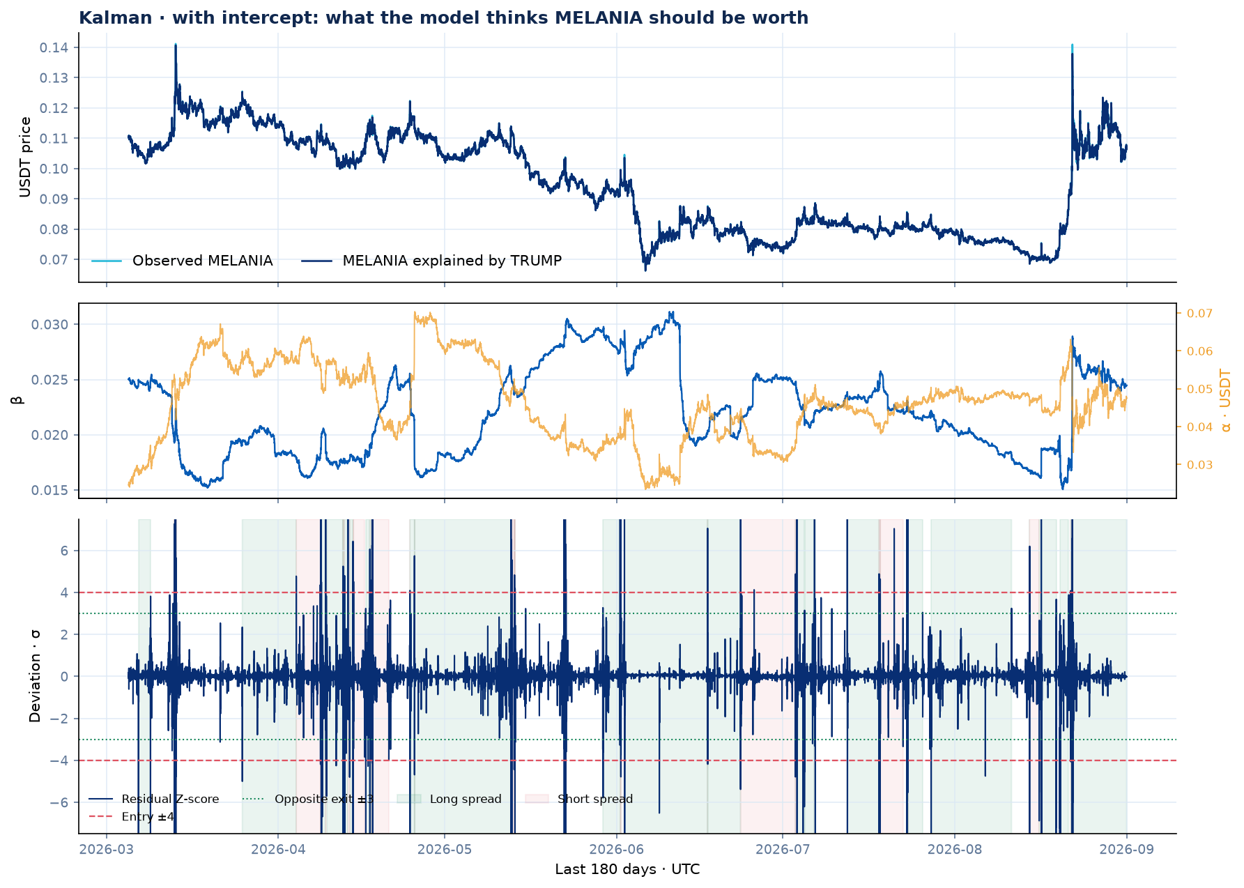
It allows both αt and βt. It is the most flexible—and the easiest to overexcite. Flexibility does not automatically mean truth.
Exact configuration and meaning of each parameter
| Model or layer | Parameter used | What it represents | What happens when it increases |
|---|---|---|---|
| OLS · without intercept | β window = 14 days 1,344 bars | Recent history used to calculate a single slope β, forcing the line through the origin. | The slope becomes smoother and more stable, but takes longer to recognise a change in the relationship. |
| OLS · with intercept | α and β window = 14 days 1,344 bars | The same sample simultaneously estimates the level α and slope β. | α and β vary less; in exchange, the model may retain an outdated relationship for longer. |
| Kalman · without intercept | qβ = 3·10−8 | Process variance of β: the amount of freedom the slope receives to change between two bars. | β reacts faster, but may also chase temporary moves. Such a small q deliberately imposes slow adaptation. |
| Kalman · with intercept | qβ = 3·10−6 qα = 3·10−8 | β can adapt more freely; α remains more rigid so the baseline does not absorb every surprise. | Increasing qβ makes the hedge more mobile; increasing qα allows the baseline to move more. Too much of both can erase the residual. |
| Kalman noise | EMA = 5 bars 75 minutes | Memory used to update the variance of the surprises observed by the filter. | Longer memory smooths the noise estimate; shorter memory reacts sooner to turbulent episodes. |
| Normalisation | Z window = 14 days 1,344 bars | Period that defines what counts as a normal or extraordinary residual. | The Z-score becomes slower and compares the present with a longer history. |
| Entry | |Z| = 4 | A position opens only when the residual reaches four standard deviations from its rolling reference. | The threshold still requires large deviations, although there is also a risk of mistaking a structural break for an opportunity. |
| Opposite-side exit | |Z| = 3 on the other side | A long opened at −4 closes at +3; a short opened at +4 closes at −3. It does not close on touching zero. | Requiring a rotation to the opposite side seeks to capture a wide move, but extends both the duration and risk of the position. |
A window and q are not the same unit. OLS explicitly remembers 14 days and abruptly forgets what came before. Kalman has no rectangular window: it retains the previous state, while q determines how much it may correct it. That is why “14 days” and “3·10−8” must not be placed on a common scale as though they were equivalent quantities.
To avoid numerical problems, the filters work with both prices divided by their first common observation. The q values refer to that normalised space. α and β are then transformed back into real prices and units to construct the residual and both legs.
These are not four independent alphas. They are four formulations of the same hypothesis. Comparing them reveals how much the deviation depends on the chosen way of estimating the relationship.
4.1OLS without intercept · the proportional agreement
4.2OLS with intercept · one additional clause
4.3Kalman without intercept · the slope learns live
4.4Kalman with intercept · everything moves
From residual to trade
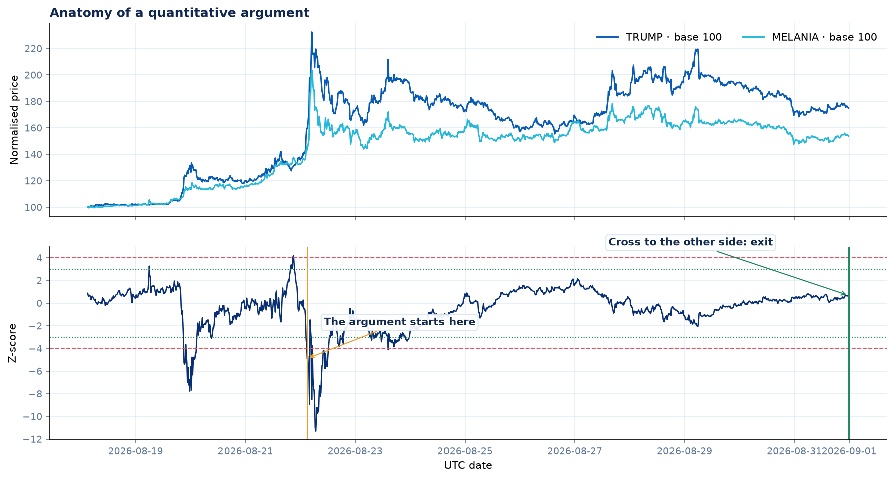
5How a statistical distance becomes two orders
Signal and execution conventions
Zero lag / current state
Each bar open updates the relationship, residual, normalisation and score before the decision on that same update. No artificial one-bar delay is added. A live implementation would still place a market-microstructure and execution filter between the score and any order.
Bid–Ask Crossing Floor
Every entry and exit pays at least the mechanical crossing cost on both legs. Where historical bid/ask quotes are unavailable, the contractual tick supplies the executable floor. This is not slippage, and it is charged once in realised PnL.
Same-bar re-entry
The existing position closes first. If the opposite entry condition is also met on the same update, a new position may open without a fictitious empty bar. The full exit and new-entry costs remain.
What it does not model: latency, queue position, market impact, partial fills, exchange outages, funding, or the intrabar path in full detail. These transparent bar-based conventions are inspectable, but they are not deployment evidence and do not promise the PnL that will reach an account.
Cointegration and reversion
6Is there an anchor—or merely two charts that look alike?
Correlation means that two series often move together. Cointegration requires something stronger: a combination of the two whose deviation remains bounded or returns to equilibrium. For pairs trading, that is the interesting property.
Engle–Granger
It estimates a relationship and applies a unit-root test to the residual. It is intuitive and natural for two assets, but depends on which one is assigned to Y and on the relationship being sufficiently stable.
Johansen
It treats the variables jointly and can detect the cointegration rank. It is more general, but sensitive to lags, trend, and sample size.
ADF + KPSS
ADF attempts to reject a unit root; KPSS attempts to reject stationarity. Using both avoids pretending that one test holds the absolute truth.
Half-life, ACF, and crossings
They measure the speed and practical behaviour of reversion. They are useful diagnostics, not notarised certificates of cointegration.
What TRUMP and MELANIA say
| Method | Null hypothesis | p-value | Reading |
|---|---|---|---|
| Engle–Granger | There is no cointegration | 0.101 | Does not reject at 5% |
| Residual ADF | The residual has a unit root | 0.031 | Rejects at 5% |
| Residual KPSS | The residual is stationary | 0.010 | Rejects stationarity |
| Johansen · rank 0 | No cointegrating vector exists | — | Rejects at 5% |
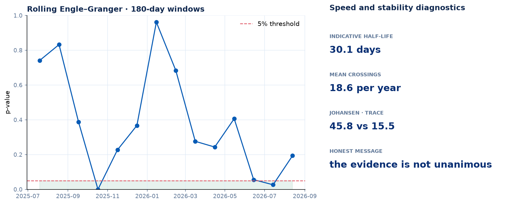
Didactic conclusion: the evidence is mixed. Engle–Granger does not reject the absence of cointegration at 5%, ADF does detect reversion in its residual, KPSS rejects stationarity, and Johansen finds one vector. This is not an error; it is a warning about instability. Cointegration is not a marriage certificate—at best, it is an interview with references.
Economic exercise
7What if we trade all four versions under exactly the same rules?
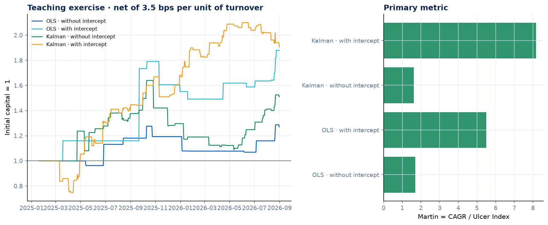
To complete the intuition, we run a simple exercise: fixed parameters, no optimisation, 3.5 basis points per unit of turnover, and the Martin ratio as the primary metric. It is neither a strategy selection nor a promise of returns.
An entry threshold of 4 expands the sample, but does not turn the example into validation. The four formulations may still generate very different trade counts because they do not construct the same residual. Entry counts must be read alongside CAGR and Martin: a few fortunate trades are not sufficient evidence.
Results ranked by Martin
The first column identifies the model. Total turnover is expressed in multiples of capital: 23× means that cumulative notional equal to 23 times capital was traded over the full sample. Average daily turnover is a percentage: it divides that turnover across all observed days. A complete entry consumes approximately 1× and its exit another 1×; a direct reversal from long to short consumes 2×. Trades counts entries initiated by the state machine.
| Model | Martin · CAGR/UI | Net CAGR | Daily Sharpe | Max drawdown | Trades | Total turnover | Average daily turnover |
|---|---|---|---|---|---|---|---|
| Kalman · with intercept | 8.16 | 49.1% | 1.42 | −25.3% | 249 | 497× | 84.3% |
| OLS · with intercept | 5.50 | 47.9% | 1.05 | −16.7% | 14 | 27× | 4.5% |
| OLS · without intercept | 1.70 | 16.0% | 0.76 | −16.2% | 12 | 23× | 3.8% |
| Kalman · without intercept | 1.62 | 29.1% | 0.82 | −33.7% | 49 | 98× | 16.6% |
Why Martin: it divides annualised return by the Ulcer Index, which measures the depth and persistence of drawdowns. Sharpe remains as context, but Martin better describes whether the path to profit was bearable—or a collection of ulcers with a chart.
What happened inside each trade: MAE and MFE
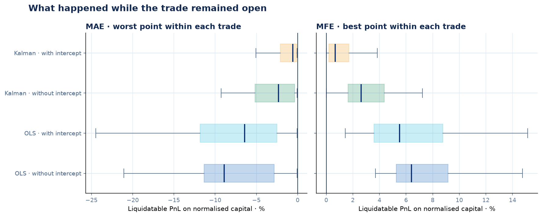
MAE (maximum adverse excursion) is the worst liquidatable PnL reached before exit: how much the trade hurt while it remained open. MFE (maximum favourable excursion) is the best liquidatable PnL reached before exit: how favourable it became, even if the eventual exit gave part of the move back.
| Model | Closed trades | Median MAE | Median MFE | Median duration | Same-bar re-entries |
|---|---|---|---|---|---|
| OLS · without intercept | 12 | −8.9% | 6.4% | 22.3 days | 0 |
| OLS · with intercept | 14 | −6.4% | 5.5% | 18.8 days | 1 |
| Kalman · without intercept | 49 | −2.3% | 2.6% | 4.8 days | 19 |
| Kalman · with intercept | 249 | −0.6% | 0.7% | 0.1 days | 178 |
What this shows—and what it does not
8The difference between a useful explanation and selling smoke with two lines
What this document does show
How the residual is constructed; what changes when an intercept is added; how Kalman adapts β; how the Z-score triggers orders; and why statistical tests may disagree.
What this document does not show
That TRUMP/MELANIA is tradable, that the parameters are robust, that the result survives other periods, or that real execution reproduces the simulation.
What the next level would require
The right idea is not “I found a pair.” It is: “I defined a convergent object, measured when it deviates, and designed an honest way to try to refute it.”
Pocket glossary
9So we can return in a year without rereading the chat
Pairs trading. A simultaneous long and short position designed to monetise a relative move.
Hedge ratio β. Proportion of leg X used to hedge one unit of leg Y.
Intercept α. Constant or dynamic level that shifts the line away from the origin.
Residual. Observed price minus the price explained by the relationship.
Z-score. Residual expressed in standard deviations relative to its rolling history.
Cointegration. Existence of a combination of non-stationary series that is itself stationary.
Half-life. Estimated time for a deviation to reduce its distance from equilibrium by roughly half.
Kalman q. Freedom granted to the state to change; more q means faster adaptation and a greater risk of chasing noise.
Turnover. Notional traded when positions change. It is expressed as a multiple of capital in total and as a percentage of capital in the daily average. This is where commissions live.
Martin ratio. CAGR divided by the Ulcer Index: return relative to the accumulated pain of drawdowns.
Sources and references
GitHub
Code, notebook and reproducible materials.
The public repository preserves the notebook, implementation and reproducible materials. This web publication retains the complete methodology, formulas, figures, results, limitations and conclusion.
GitHub Code and reproduction