Executive result

A real gross effect. An untradeable net result.

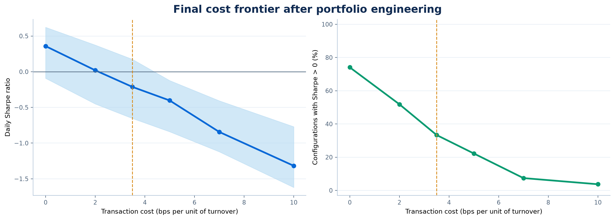
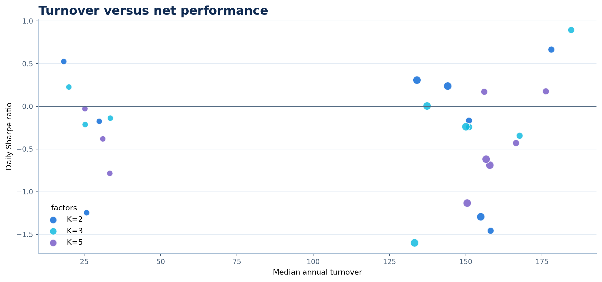
Residual dislocations revert often enough to produce a positive gross signal. The problem is economic, not cosmetic: capturing it requires so much trading that the result crosses below zero between 0 and 2 basis points per unit of turnover.

0.358Final median gross Sharpe

74.1%Final grid positive gross

150.1×Median annual turnover

−0.213Median Sharpe at 3.5 bps

Decision: close this 15-minute PCA-residual branch and move to funding carry. No isolated best configuration is allowed to overrule the pre-registered median-of-grid criterion.

Research question

Can relative mispricing survive after common crypto risk is removed?

The market often moves as one large risk complex. A token can rise while still underperforming what its exposure to the common market factors would imply. The study asks whether that idiosyncratic gap subsequently converges strongly enough to trade.

The object that converges

Not a bilateral pair. It is each asset’s cumulative return residual after projecting out a small set of rolling PCA factors.

The economic bet

Buy unusually negative residuals and sell unusually positive residuals while constraining the portfolio’s common-factor exposure.

The falsification test

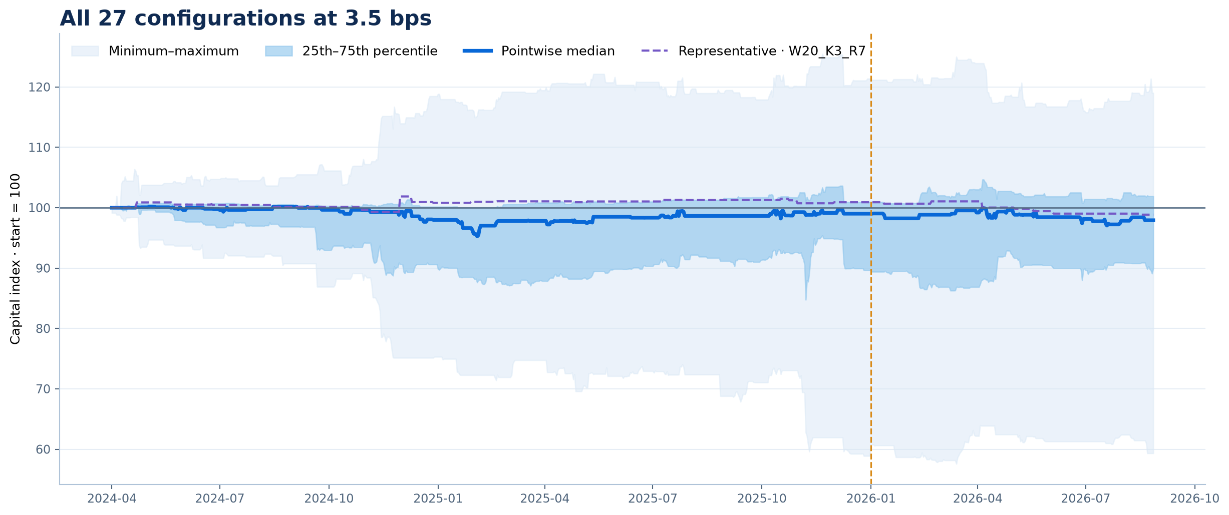
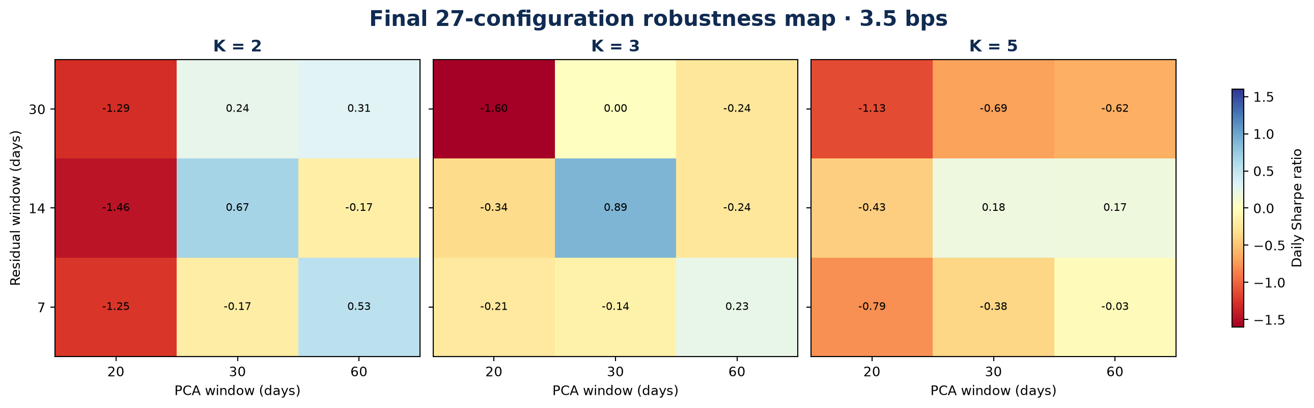
The broad grid—not its maximum—must remain positive after 3.5 bps per unit of turnover and across time.

“A backtest is useful when it can kill an attractive story before capital has to.”

Experimental design

One chronological research programme, two stages

Version 1.0 established whether the phenomenon existed. Version 1.1 tested the cheapest plausible fixes to the turnover problem without changing the hypothesis after seeing the answer.

Observe

50 liquid USDT perpetuals, aligned 15-minute opens.

Neutralize

Estimate rolling PCA factors and isolate residual returns out of sample.

Standardize

Accumulate residuals and map their deviation to an OU-style score.

Construct

Contrarian, factor-neutral weights with explicit portfolio turnover.

Falsify

Stress costs, time periods and a pre-defined continuation grid.

Data. OKX USDT-margined perpetual swaps; 50 instruments; 15-minute bars built from 1-minute opens; common evaluation from 1 April 2024 to 27 August 2026. The repository excludes raw exchange data.

Execution convention. Signals and portfolio weights act at time t. This bar-level study is a screening experiment—not a claim that bar data can reproduce live order-book execution.

Method

From prices to a neutral residual portfolio

The method is deliberately linear and interpretable. Each transformation has a specific job and can be inspected independently.

Convert open prices to log returns

rᵢ,ₜ = log(Pᵢ,ₜ / Pᵢ,ₜ₋₁)

Missing or structurally stale instruments are excluded from the relevant rolling estimate rather than filled with invented returns.

Estimate common factors on a rolling window

Cₜ = corr(Rₜ₋W:ₜ), CₜVₜ = VₜΛₜ

PCA is applied to the correlation matrix, preventing high-volatility assets from mechanically dominating. Marchenko–Pastur is used as a diagnostic of how many eigenvalues rise above a noise benchmark.

Generate out-of-sample residual returns

εₜ = Zₜ − ZₜVₜVₜ⊤

Loadings are frozen between refreshes. The next block is transformed with parameters estimated only from prior observations, avoiding look-ahead.

Build and score the residual state

Xᵢ,ₜ = Σ εᵢ,ᵤ, ΔXₜ = a + bXₜ₋₁ + ηₜ

The accumulated residual is evaluated with an AR(1)/Ornstein–Uhlenbeck representation. Entry thresholds select unusually displaced states; the position is contrarian.

Neutralize and charge the actual portfolio movement

min_w ||w − w*||² subject to B⊤w ≈ 0, Σ|w| = 1

costₜ = c · Σᵢ|wᵢ,ₜ − wᵢ,ₜ₋₁|

Factor legs are netted at portfolio level. Costs are charged on final-weight turnover; the same factor hedge is never counted twice.

Why the PCA regression can be simplified exactly

With standardized returns Z and orthonormal eigenvectors V, factors are F = ZV. The OLS beta of Z on F is (F′F)⁻¹F′Z = V′. Thus projection with VV′ is algebraically identical to recomputing the regression and is cheaper and more stable.

Risk and performance statistics

Performance is aggregated daily before annualizing Sharpe to absorb intraday dependence. The report also tracks Sortino, Calmar, Martin ratio, drawdown, CAGR, turnover, holding time, fraction of positive configurations and the grid median. The last two prevent a lucky maximum from masquerading as robustness.

Stage I · Baseline v1.0

The first grid found signal—and immediately exposed its fragility

The 81-configuration grid crossed three PCA windows, three factor counts, three residual horizons and three entry thresholds. It asked whether a broad region of the model behaved well, not which single row looked best.

Baseline parameter grid.
Dimension	Values	Purpose
PCA lookback	20 / 30 / 60 days	Factor stability versus adaptation
Factors K	2 / 3 / 5	Amount of common variation removed
Residual horizon	7 / 14 / 30 days	State and OU estimation horizon
Entry score	1.5 / 2.0 / 2.5	Trade frequency versus extremeness

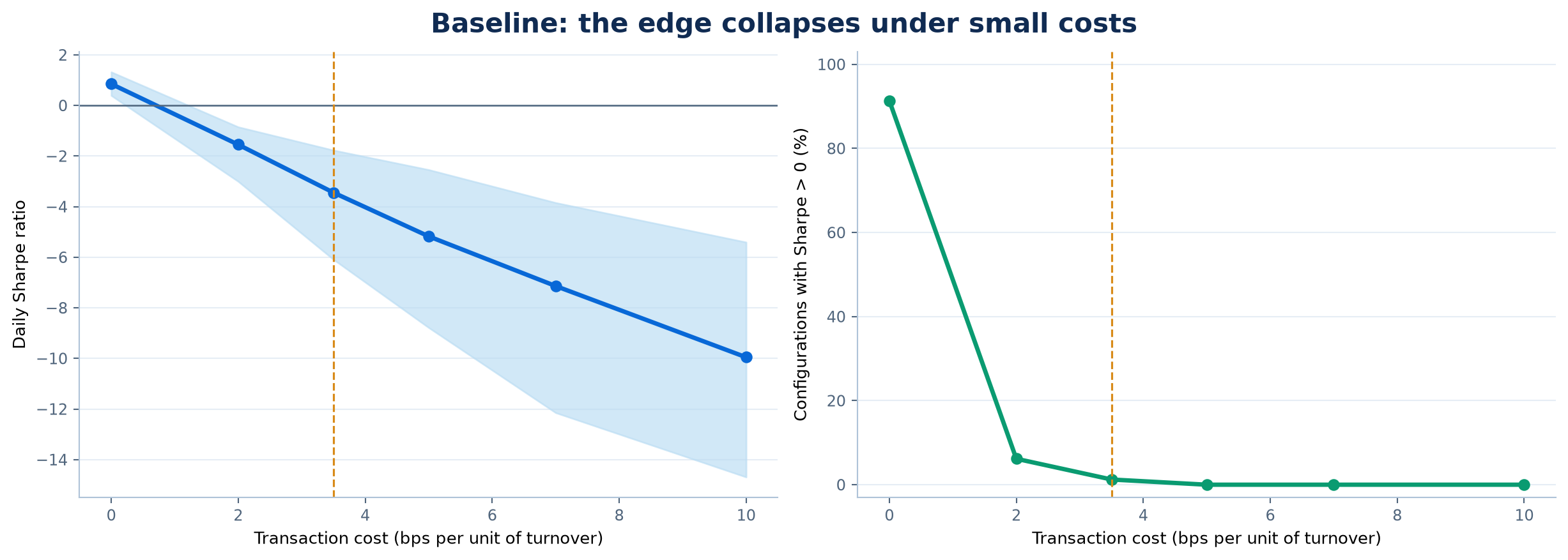
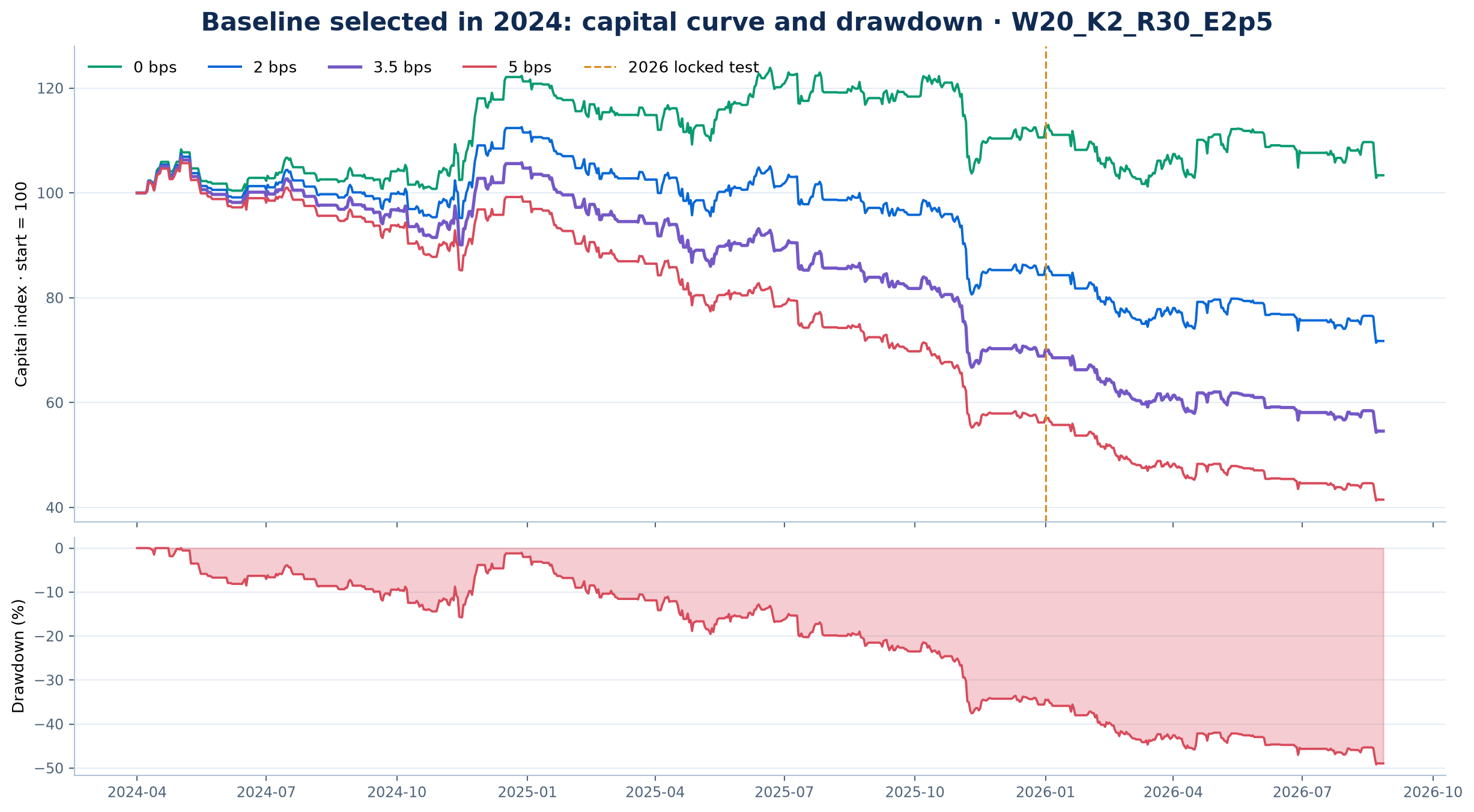
Baseline median Sharpe and positive grid fraction across transaction costs — **Figure 1.** At zero cost, 91.4% of the grid is positive. At 3.5 bps, only 1.2% remains positive and the median Sharpe falls to −3.44. The dashed line is the governance cost.

Equity curves of the selected baseline configuration under multiple costs — **Figure 2.** The baseline’s selected representative configuration (20-day PCA, two factors, 30-day residual state, 2.5 entry threshold) is not temporally stable after costs: 2025 Sharpe is −2.42 and 2026 Sharpe is −1.93 at 3.5 bps.

Diagnosis, not conclusion: residual reversion appears in gross returns, but concentration reached roughly 50% in one asset and turnover was extreme. That justified one bounded continuation—not indefinite parameter rescue.

Stage II · Continuation v1.1

Four levers were allowed. Each had a reason and a stopping rule.

The continuation was specified before execution. Cheap interventions stayed within the hypothesis; lower-frequency reformulations and explicit BTC factors were classified as new projects, not post-hoc repairs.

A · Weight caps

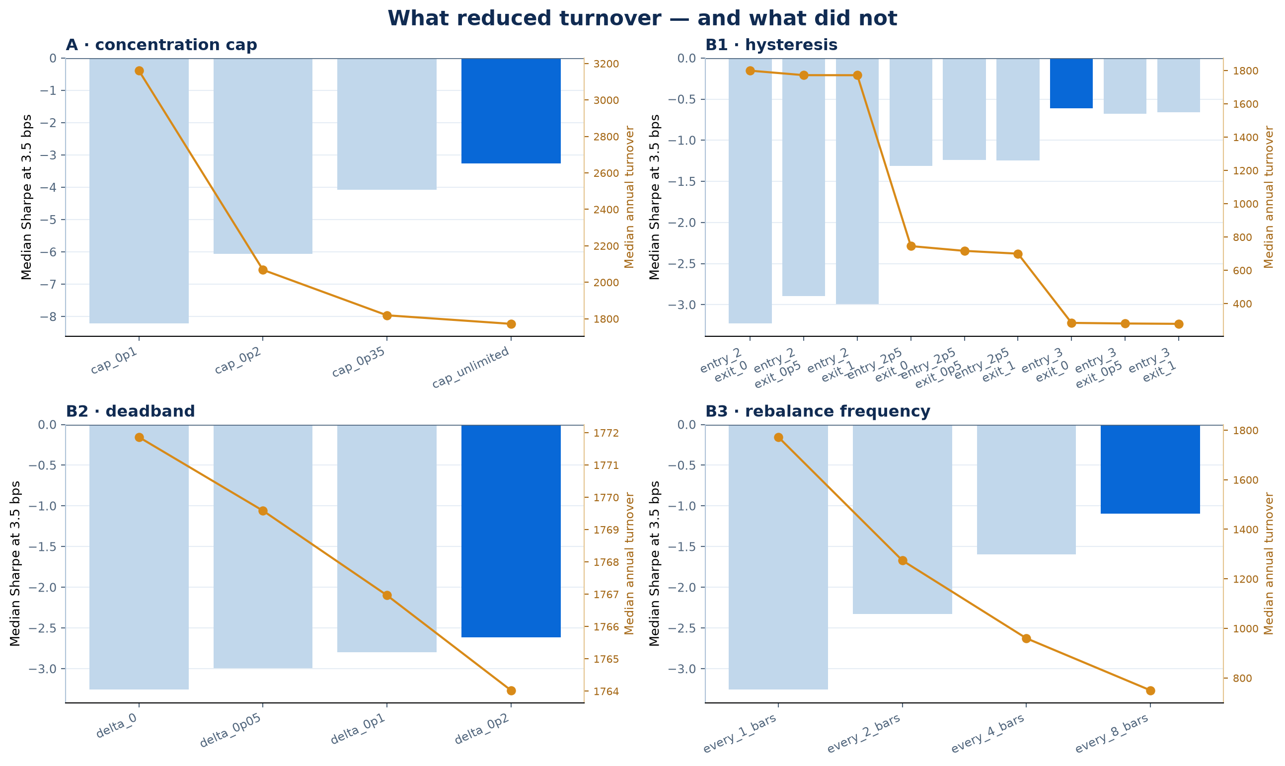
Cap each asset at 10%, 20% or 35% to attack the 50% concentration observed in the baseline.

B1/B2/B3 · Trading inertia

Wider entry/exit hysteresis, a no-trade deadband and action every 1, 2, 4 or 8 bars.

B4 · Turnover penalty

Penalize movement inside portfolio construction instead of projecting first and paying later.

C · Residual-quality filters

Trade only the top 75%, 50% or 25% of residual series by AR(1) fit quality.

Frozen final recipe

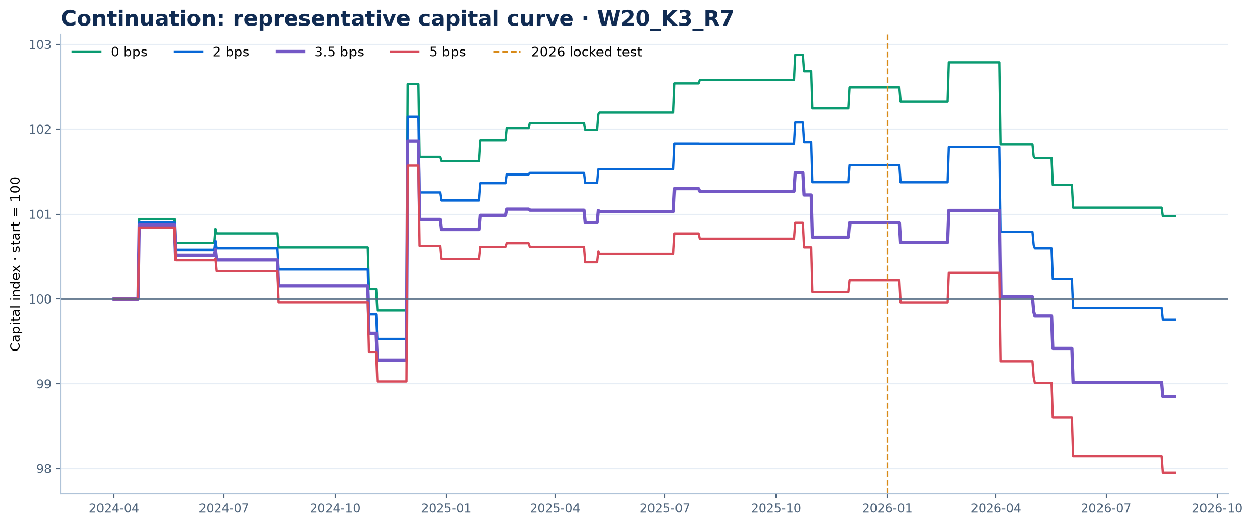
No cap; entry 3; exit 0; 0.2 deadband; act every 8 bars; no movement penalty; all eligible residuals.

Effect of continuation interventions on Sharpe and turnover — **Figure 3.** Acting less often and demanding larger deviations reduced turnover materially. Caps worsened the result, tiny deadbands barely mattered, and positive turnover penalties largely immobilized the book.

Representative continuation equity curves — **Figure 4.** Representative final configuration under multiple transaction costs.

Distribution envelope of final grid equity curves — **Figure 5.** The median and interquartile envelope reveal the grid, preventing attention from drifting to one unusually good path.

Final grid Sharpe and positive fraction by cost — **Figure 6.** Engineering moved the cost frontier: at 2 bps, the median is approximately flat and 51.9% of configurations are positive. At the locked 3.5 bps, the median is −0.213 and only 33.3% are positive.

Robustness

The answer must survive configuration choice, trading intensity and time

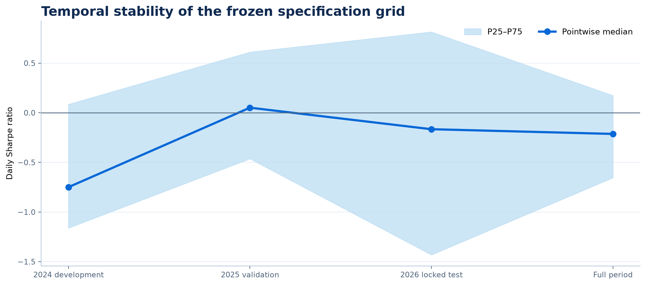
A credible research decision cannot depend on one backtest curve. The final assessment uses a 27-configuration grid, a turnover frontier and time-sliced validation.

Heatmap of final grid Sharpe at 3.5 basis points — **Figure 7.** Final 27-configuration robustness grid. The failure is a broad surface, not a single bad parameter choice.

Turnover versus net Sharpe frontier — **Figure 8.** Lower turnover helps, but no stable low-turnover region clears the governance bar.

Sharpe by validation subperiod — **Figure 9.** Subperiod results show why the full-period statistic is not sufficient evidence of durability.

Final-grid cost robustness.
Cost	Median Sharpe	Positive grid	Interpretation
0 bps	0.358	74.1%	Statistical phenomenon exists gross
2.0 bps	≈ 0.020	51.9%	Economic edge nearly exhausted
3.5 bps	−0.213	33.3%	Locked acceptance test fails

Conclusion

What this study proves—and what it does not

The negative decision is the product. It preserves research capital and narrows the next question.

Supported by the evidence

PCA residual dislocations contain measurable short-horizon mean reversion.
The gross effect is broad across the final grid.
Slower action and stronger thresholds reduce turnover.
At the chosen market-friction assumption, the 15-minute implementation is not robustly profitable.

Not established

That residual reversion is absent at 1-hour or 4-hour horizons.
That an explicit BTC or sector factor model cannot improve residual quality.
That order-book execution would recover the missing economics.
That the result transfers unchanged to another exchange, universe or fee tier.

Next branch: funding and basis carry, where the convergence anchor is mechanical and turnover is naturally lower. Slow residual models remain separate new hypotheses, not a continuation of this grid.

Open research package

Reproduce the pipeline without redistributing exchange data

The repository contains research code, locked configurations, figure generation and methodological documentation. Raw OKX candles are deliberately excluded; the data guide explains how to obtain and transform them.

Public repository

Clone the project, follow the data contract, run the baseline and continuation, then regenerate every figure from the aggregated artifacts.

View on GitHub →

Data and sources

Provenance and transformations

Instruments were identified from OKX’s public swap catalogue, and candles came from its official historical-candles endpoint. Snapshot end: 27 August 2026, 23:45 UTC.

The study uses the first open of each 15-minute interval, built from 1-minute opens. Raw exchange data are not redistributed; the public repository retains the code, configuration, and aggregated artifacts.

1 · Acquire

Download 1-minute OKX perpetual candles and aggregate each 15-minute bar with the first open.

2 · Research

Run the time-causal factor-residual pipeline using the committed parameter registry.

3 · Audit

Compare the grid medians, positive fractions and subperiod metrics—not just the maximum Sharpe.

Limitations and scope

Survivorship effects, exchange-specific instrument availability, bar-level execution, omission of funding in the initial price-only experiment and model drift all limit external validity. Costs are expressed as scenarios rather than claimed as universal realized slippage. This is research, not investment advice.

How to cite

Barredo Lago, Carlos (2026). “Factor-Residual Reversion in Crypto Perpetuals: A Cost-Aware Falsification Study.” Qinvia Research. Source and citation metadata are included in the repository.

Factor-residual reversion in crypto perpetuals

The study at a glance